Chapter 15 of 25
Activation Functions
The spark that lets networks learn anything non-linear
25 min read
Created ২ আগ, ২০২৬
ভূমিকা (Motivation)
গত চ্যাপ্টারে আপনি ইতিমধ্যে একটি গুরুত্বপূর্ণ জিনিস প্রমাণ করে ফেলেছেন: আপনি চাইলে পর পর যত খুশি লিনিয়ার লেয়ার সাজাতে পারেন, কিন্তু দিনশেষে আপনি শুধু একটি সরলরেখাই (বা সমতল পৃষ্ঠ বা ফ্ল্যাট প্লেন) পাবেন। এই অভিশাপ ভাঙার একমাত্র জিনিসটি — অর্থাৎ সেই একক উপাদানটি যা গভীরতা বা ডেপথ (depth) বাড়িয়ে আসলে কাজের কাজ কিছু একটা করে — তা হলো সেই ছোট্ট ননলিনিয়ার (nonlinear) ফাংশনটি, যাকে প্রতিটি নিউরনের ভেতর ঠিক ওয়েটেড সামের পরেই বসিয়ে দেওয়া হয়। ওই ফাংশনটিকে বলা হয় অ্যাক্টিভেশন ফাংশন (activation function), আর এই চ্যাপ্টারটি হলো বাস্তবে ব্যবহৃত হওয়া অ্যাক্টিভেশন ফাংশনগুলোর একটি সম্পূর্ণ ট্যুর। এর মধ্যে এটাও থাকবে যে কেন কিছু ফাংশন সময়ের সাথে বাতিল হয়ে গেছে এবং কেন অন্যগুলো প্রায় সব জায়গাতেই ডিফল্ট পছন্দ হয়ে দাঁড়িয়েছে।
একটি বাস্তব জীবনের উদাহরণ (A Real-Life Scenario)
ভাবুন তো, একটি সাধারণ থার্মোস্ট্যাট (thermostat) কীভাবে কাজ করে আর একটি স্মার্ট ক্লাইমেট সিস্টেম (smart climate system) কীভাবে কাজ করে। একটি বোকা থার্মোস্ট্যাট মূলত একটি স্টেপ ফাংশনের (step function) মতো কাজ করে: তাপমাত্রা টার্গেটের নিচে থাকলে হিটার পুরো দমে চালু; আর ওপরে গেলে পুরোপুরি বন্ধ। এটা খুব সহজ, কিন্তু বেশ হুট করে বদলে যায় এবং এতে কোনো বিস্তারিত তথ্য থাকে না — এটি আপনাকে কখনোই বোঝায় না যে আপনি টার্গেটের ঠিক কতটা কাছাকাছি আছেন, আর এমন শুধু অন-অফ সুইচের ওপর ভিত্তি করে তৈরি কোনো কন্ট্রোল সিস্টেম খুব ঝাঁকুনি দিয়ে চলবে এবং তাকে সূক্ষ্মভাবে টিউন করা প্রায় অসম্ভব হয়ে দাঁড়াবে।
এর বদলে একটি স্মার্ট সিস্টেম খুব মসৃণভাবে সাড়া দেয়: রুম যত ঠান্ডা হতে থাকে, সে হিটারকে ধীরে ধীরে তত বাড়াতে থাকে, আর রুম গরম হতে থাকলে সে ধীরে ধীরে হিটার কমিয়ে আনে। ওই মসৃণ এবং ধীরে ধীরে বদল হওয়া রেসপন্সটিই আধুনিক অ্যাক্টিভেশন ফাংশনগুলো একটি Neural Network-এর ভেতরে অর্জন করার চেষ্টা করে — অর্থাৎ ইনপুটের বিপরীতে শুধু "পুরোপুরি চালু" বা "পুরোপুরি বন্ধ" না হয়ে এমনভাবে রেসপন্স করা, যা একটি নিরবচ্ছিন্ন ও তথ্যবহুল গ্রেডিয়েন্ট বহন করে এবং যা থেকে নেটওয়ার্কটি শিখতে পারে।
মূল ধারণা তৈরি করা (Building the Intuition)
- প্রতিটি অ্যাক্টিভেশন ফাংশন একটি raw ওয়েটেড সাম () নেয় এবং পরের লেয়ারে পাঠানোর আগে তাকে কোনো না কোনো ননলিনিয়ার উপায়ে চেপে দেয়, আকার পালটে দেয় অথবা ফিল্টার করে।
- একটি ভালো অ্যাক্টিভেশন ফাংশনকে অবশ্যই ননলিনিয়ার (nonlinear) হতে হবে (নইলে ডেপথ বাড়িয়ে কোনো লাভ নেই, যা আমরা গত চ্যাপ্টারে প্রমাণ করেছি), (প্রায় সব জায়গায়) ডিফারেনশিয়েবল (differentiable) বা অন্তরীকরণযোগ্য হতে হবে (যাতে backpropagation কাজ করার জন্য একটি গ্রেডিয়েন্ট পায়), কম্পিউট করার জন্য খুব সস্তা হতে হবে (কারণ এটি প্রতি ট্রেনিং স্টেপে মিলিয়ন মিলিয়ন বার রান হয়), এবং আদর্শগতভাবে এটিকে স্যাচুরেটিং (saturating) হওয়া এড়াতে হবে — অর্থাৎ ইনপুটের বিশাল একটা অংশ জুড়ে ডেরিভেটিভ যেন শূন্যের কাছাকাছি না হয়ে যায়।
- এই শেষ বৈশিষ্ট্যটি, অর্থাৎ স্যাচুরেশন, আদতে এই পুরো চ্যাপ্টারের মূল বিষয়। ঠিক এই কারণেই সিগময়েড (sigmoid) এবং ট্যানএইচ (tanh), যা একসময় সবার প্রথম পছন্দ ছিল, তা আজ অনেকাংশেই বাতিল হয়ে গিয়ে তার জায়গা দখল করে নিয়েছে ReLU এবং তার বংশধরেরা।
ভ্যানিশিং এবং এক্সপ্লোডিং গ্রেডিয়েন্ট সমস্যা (The Vanishing and Exploding Gradient Problem)
Backpropagation-এর সময়, এরর সিগন্যাল (error signal) -কে পেছনের দিকে প্রবাহিত হওয়ার সময় প্রতিটি একক লেয়ারে দিয়ে গুণ করা হয়। যদি ধারাবাহিকভাবে 1-এর চেয়ে অনেক ছোট হয় (যেমনটা সিগময়েড এবং ট্যানএইচ স্যাচুরেট হয়ে গেলে হয়), তবে এই বারবার গুণ হওয়ার ফলে গ্রেডিয়েন্টটি যত পেছনের দিকে যায়, তত দ্রুত এক্সপোনেনশিয়ালি (exponentially) কমতে থাকে — একে বলা হয় ভ্যানিশিং গ্রেডিয়েন্ট প্রবলেম (vanishing gradient problem)। এর ফলে একটি গভীর বা ডিপ নেটওয়ার্কের শুরুর দিকের লেয়ারগুলো বলতে গেলে শেখার মতো কোনো সিগন্যালই পায় না এবং কার্যকরভাবে তাদের উন্নতি হওয়া পুরোপুরি থেমে যায়। এর ঠিক উল্টো আরেকটি ব্যর্থতা ঘটে, যেখানে যদি ধারাবাহিকভাবে 1-এর চেয়ে বড় হয়, তখন গ্রেডিয়েন্টগুলো কমার বদলে এক্সপোনেনশিয়ালি বাড়তে থাকে এবং ফেটে পড়ে — একে বলা হয় এক্সপ্লোডিং গ্রেডিয়েন্ট প্রবলেম (exploding gradient problem)।
এই একটি সমস্যাই Deep Learning-এর দশকের পর দশকের ইতিহাস বদলে দিয়েছে
ভ্যানিশিং গ্রেডিয়েন্ট ছিল সত্যিকার অর্থে গভীর বা ডিপ নেটওয়ার্ক ট্রেন করার পথে বছরের পর বছর ধরে প্রধান একটি প্র্যাক্টিক্যাল বাধা। হিডেন লেয়ারের (hidden layers) জন্য কেন ReLU-ফ্যামিলির অ্যাক্টিভেশনগুলো সবার ডিফল্ট পছন্দ হয়ে উঠল, তা বুঝতে হলে এই মেকানিজমটি বোঝা অত্যন্ত জরুরি।
এর পেছনের গণিত: অ্যাক্টিভেশন ফাংশনগুলোর তালিকা (The Math Behind It: A Catalog of Activation Functions)
বাইনারি স্টেপ (ঐতিহাসিক) (Binary Step)
অরিজিনাল perceptron ঠিক এটাই ব্যবহার করত। এর গ্রেডিয়েন্ট প্রায় সব জায়গাতেই শূন্য (zero), যা একে গ্রেডিয়েন্ট-ভিত্তিক লার্নিংয়ের জন্য পুরোপুরি অকেজো করে তোলে — এটি এখন শুধুই একটি ঐতিহাসিক উদাহরণ হিসেবে বেঁচে আছে।
সিগময়েড (লজিস্টিক) (Sigmoid / Logistic)
ডেরিভেটিভ প্রতিপাদন: ধরি , সুতরাং । চেইন রুল অনুসারে, । যেহেতু , তাই এর মান বসালে এবং সরল করলে পাওয়া যায় ।
রেঞ্জ: । সুবিধাসমূহ: মসৃণ (smooth), সরাসরি প্রোবাবিলিটি হিসেবে ব্যাখ্যা করা যায়, ঐতিহাসিকভাবে বেশ গুরুত্বপূর্ণ। অসুবিধাসমূহ: বড় -এর জন্য স্যাচুরেট করে — এর সর্বোচ্চ ডেরিভেটিভ মাত্র , যা -তে পাওয়া যায় — ফলে ডিপ নেটওয়ার্কগুলোতে তীব্র ভ্যানিশিং গ্রেডিয়েন্ট তৈরি করে; এর আউটপুট জিরো-সেন্টারড (zero-centered) নয়, যা কনভার্জেন্স (convergence) ধীর করে দিতে পারে। ব্যবহারের ক্ষেত্র: বাইনারি ক্লাসিফিকেশনের আউটপুট লেয়ারে (আউটপুটটিকে হিসেবে ব্যাখ্যা করার জন্য); আধুনিক ডিপ নেটওয়ার্কের হিডেন লেয়ারে এর ব্যবহার খুবই বিরল।
হাইপারবোলিক ট্যানজেন্ট (ট্যানএইচ) (Hyperbolic Tangent / Tanh)
রেঞ্জ: । সুবিধাসমূহ: জিরো-সেন্টারড (সিগময়েডের মতো নয়), যা সাধারণত কনভার্জেন্স স্পিড বাড়ায়, এবং শূন্যের কাছাকাছি এর গ্রেডিয়েন্ট অপেক্ষাকৃত বেশি খাড়া। অসুবিধাসমূহ: বড় -এর জন্য এটি এখনও স্যাচুরেট করে, তাই ডিপ নেটওয়ার্কগুলোতে এটিও ভ্যানিশিং গ্রেডিয়েন্টের শিকার হয়। ব্যবহারের ক্ষেত্র: ReLU স্ট্যান্ডার্ড হওয়ার আগে হিডেন লেয়ারগুলোতে ঐতিহাসিকভাবে বেশ প্রচলিত ছিল; এখনও কিছু রিকারেন্ট (recurrent) আর্কিটেকচারে দেখা যায়।
রেলু বা রেক্টিফাইড লিনিয়ার ইউনিট (ReLU / Rectified Linear Unit)
রেঞ্জ: । সুবিধাসমূহ: কম্পিউট করা খুবই সস্তা; প্রতিটি পজিটিভ ইনপুটের জন্য এর ডেরিভেটিভ হুবহু 1, তাই এটি পজিটিভ দিকে কখনোই স্যাচুরেট করে না, যা মূলত ওই দিকের ভ্যানিশিং গ্রেডিয়েন্টের সমাধান করে দেয়; বাস্তব ক্ষেত্রে এটি সিগময়েড বা ট্যানএইচ-এর চেয়ে অনেক দ্রুত কনভার্জ করে। অসুবিধাসমূহ: ডাইং রেলু প্রবলেম (dying ReLU problem) — ট্রেনিংয়ের সময় যদি কোনো নিউরনের প্রি-অ্যাক্টিভেশন ধারাবাহিকভাবে নেগেটিভ বা ঋণাত্মক হতে থাকে, তবে সে আজীবনের জন্য শূন্য গ্রেডিয়েন্ট পেতে শুরু করে এবং কার্যকরভাবে তার শেখা পুরোপুরি ও চিরস্থায়ীভাবে বন্ধ হয়ে যায়; এটি জিরো-সেন্টারডও নয়। ব্যবহারের ক্ষেত্র: আধুনিক বেশিরভাগ ফিডফরোয়ার্ড (feedforward) এবং কনভোল্যুশনাল (convolutional) নেটওয়ার্কের হিডেন লেয়ারের জন্য এটিই হলো ডিফল্ট পছন্দ।
ইন্টারভিউয়ের জন্য খুব পরিচিত একটি প্রশ্ন
"ডাইং রেলু প্রবলেম (dying ReLU problem) কী, এবং কীভাবে এটি কমানো যায়?" এর মেকানিজমটি বুঝিয়ে বলুন — ধারাবাহিকভাবে নেগেটিভ প্রি-অ্যাক্টিভেশন আজীবনের জন্য শূন্য গ্রেডিয়েন্ট তৈরি করে — তারপর এর সমাধানগুলো উল্লেখ করুন: Leaky ReLU, ELU, অথবা SELU (নিচে দেখুন), খুব সাবধানে ওয়েট ইনিশিয়ালাইজ (weight initialization) করা, এবং তুলনামূলক কম লার্নিং রেট (learning rates) ব্যবহার করা।
লিকি রেলু (Leaky ReLU)
যেখানে হলো একটি ছোট ধ্রুবক, সাধারণত । এটি হওয়ার সময় একটি ছোট, শূন্য নয় এমন গ্রেডিয়েন্ট দেওয়ার মাধ্যমে ডাইং রেলু প্রবলেমের সমাধান করে, তবে এর বিনিময়ে আপনাকে বেছে নেওয়ার জন্য অতিরিক্ত একটি হাইপারপ্যারামিটার (hyperparameter) যোগ করতে হয়। যখন কোনো ডাইং নিউরন ধরা পড়ে, তখন ReLU-এর সরাসরি বিকল্প বা ড্রপ-ইন রিপ্লেসমেন্ট (drop-in replacement) হিসেবে এটি খুব সাধারণ পছন্দ।
ইলু (ELU / Exponential Linear Unit)
ELU বেশ মসৃণ (Leaky ReLU-এর মতো শূন্যতে কোনো চোখা ভাঁজ নেই), এবং এর নেগেটিভ মানগুলো গড় বা মিন অ্যাক্টিভেশনকে শূন্যের কাছাকাছি ঠেলে দেয়, যা লার্নিং স্পিড বাড়িয়ে দিতে পারে — এই পেছনের যুক্তিটা অনেকটা ব্যাচ নরমালাইজেশনের (batch normalization) মতোই। তবে এর ট্রেড-অফ (trade-off) হলো এক্সপোনেনশিয়ালের কারণে হওয়া অতিরিক্ত কম্পিউটেশনাল খরচ।
সেলু (SELU / Scaled ELU)
যেখানে ফিক্সড বা নির্দিষ্ট ধ্রুবকগুলো হলো এবং (এগুলো টিউন করার মতো কোনো হাইপারপ্যারামিটার নয়)। নির্দিষ্ট কিছু শর্তে — যেমন লেকুন নরমাল (LeCun normal) ওয়েট ইনিশিয়ালাইজেশন এবং অন্য কোনো নরমালাইজেশন লেয়ার ছাড়া একটি প্লেইন ফিডফরোয়ার্ড আর্কিটেকচার — SELU প্রতিটি লেয়ারের আউটপুটকে স্বয়ংক্রিয়ভাবে শূন্য মিন (zero mean) এবং ইউনিট ভ্যারিয়েন্সের (unit variance) দিকে কনভার্জ করতে সাহায্য করে, যাকে বলা হয় সেলফ-নরমালাইজেশন (self-normalization)। তবে এর এই সুবিধাটি বেশ ভঙ্গুর: স্কিপ কানেকশন (skip connections), স্ট্যান্ডার্ড ড্রপআউট (dropout), বা ব্যাচ নরমালাইজেশন থাকলে এটি কাজ নাও করতে পারে।
সফটপ্লাস (Softplus)
এটি হলো শূন্যতে কোনো চোখা ভাঁজ না থাকা ReLU-এর একটি মসৃণ বা স্মুথ অ্যাপ্রক্সিমেশন (smooth approximation), যা সব জায়গায় ডিফারেনশিয়েবল, কিন্তু এটি কম্পিউট করা বেশ ব্যয়বহুল এবং এটি এখনও খুব বেশি নেগেটিভ ইনপুটের জন্য ছোট গ্রেডিয়েন্ট তৈরি করতে পারে।
সুইশ (Swish)
যেখানে হলো একটি ধ্রুবক বা লার্ন্যাবল (learnable) প্যারামিটার, যা অনেক সময় কেবল 1-এ ফিক্সড রাখা হয়। সুইশ বেশ মসৃণ এবং নন-মনোটোনিক (non-monotonic) — অর্থাৎ এটি শূন্যতে ফিরে আসার আগে ছোট নেগেটিভ -এর জন্য শূন্যের সামান্য নিচে নেমে যায় — এবং বাস্তব পরীক্ষায় দেখা গেছে যে এটি কিছু ডিপ আর্কিটেকচারে ReLU-কে টেক্কা দিতে পারে, তবে এর জন্য অতিরিক্ত কম্পিউটেশনাল খরচ গুনতে হয়।
জেলু (GELU / Gaussian Error Linear Unit)
যেখানে হলো স্ট্যান্ডার্ড নরমাল কিউম্যুলেটিভ ডিস্ট্রিবিউশন ফাংশন (standard normal cumulative distribution function), যাকে দ্রুত হিসাব করার জন্য প্রায়ই হিসেবে অ্যাপ্রক্সিমেট করা হয়। GELU-কে এভাবে ব্যাখ্যা করা যায় যে, এটি ইনপুটকে এমন একটি প্রোবাবিলিটি দিয়ে ওয়েট বা গুণ করে যা নির্দেশ করে যে একটি স্ট্যান্ডার্ড নরমাল ভেরিয়েবল -এর চেয়ে ছোট হওয়ার সম্ভাবনা কতটুকু, এবং এটি এখন ট্রান্সফর্মার-ভিত্তিক (Transformer-based) আর্কিটেকচারগুলোর স্ট্যান্ডার্ড অ্যাক্টিভেশন ফাংশন হয়ে দাঁড়িয়েছে।
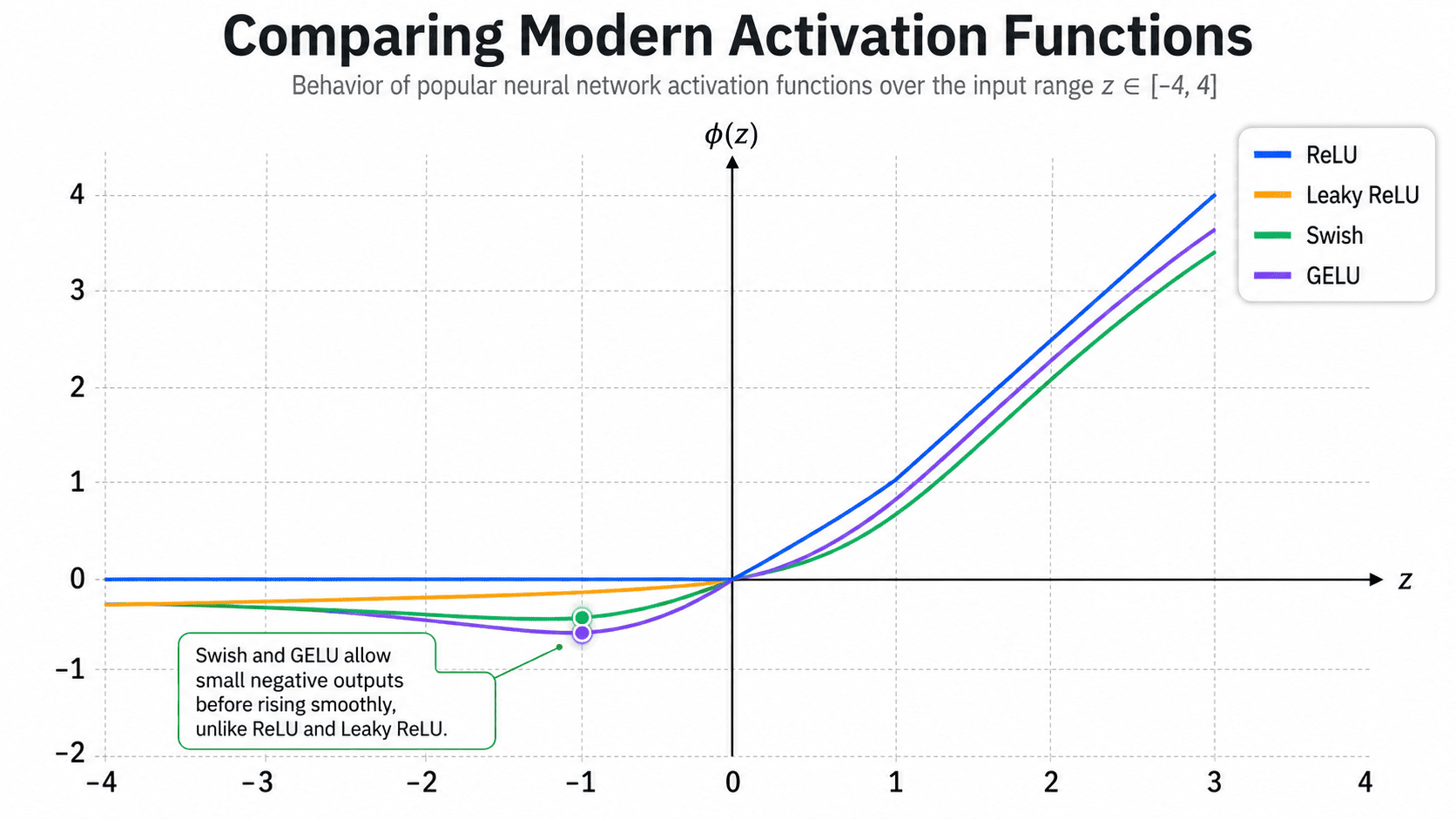
ইন্টারেক্টিভ: প্রতিটি ফাংশন এবং তার ডেরিভেটিভ এক্সপ্লোর করুন (Interactive: Explore Each Function and Its Derivative)
অ্যাক্টিভেশন ফাংশন এক্সপ্লোরার (Activation Function Explorer)
সিগময়েড, ট্যানএইচ, ReLU, অথবা Leaky ReLU বেছে নিন এবং ফাংশনটিকে তার ডেরিভেটিভের সাথে প্লট করা অবস্থায় দেখুন — খেয়াল করুন এদের প্রত্যেকে কোথায় গিয়ে স্যাচুরেট করে।
f(x)f'(x)
হাতে-কলমে সংখ্যাগত তুলনা: একই ইনপুটে সব ফাংশন (Worked Numerical Comparison: All Functions at the Same Input)
তত্ত্বকথা থেকে বেরিয়ে, চলুন একই দুটি ইনপুট, (একটি মাঝারি পজিটিভ মান) এবং (এর সমান কিন্তু নেগেটিভ প্রতিরূপ), ব্যবহার করে প্রতিটি ফাংশন সরাসরি হাতে-কলমে গণনা করে দেখি। এটি স্যাচুরেশনের প্রভাবকে বিমূর্ত আলোচনা থেকে বাস্তব সংখ্যায় নামিয়ে আনে।
| ফাংশন (Function) | φ(2.0) | φ'(2.0) | φ(-2.0) | φ'(-2.0) |
|---|---|---|---|---|
| সিগময়েড (Sigmoid) | 0.881 | 0.105 | 0.119 | 0.105 |
| ট্যানএইচ (Tanh) | 0.964 | 0.071 | -0.964 | 0.071 |
| রেলু (ReLU) | 2.0 | 1.0 | 0.0 | 0.0 |
| লিকি রেলু (Leaky ReLU, α=0.01) | 2.0 | 1.0 | -0.02 | 0.01 |
খেয়াল করুন সবচেয়ে গুরুত্বপূর্ণ প্যাটার্নটি: -এর জন্য সিগময়েড এবং ট্যানএইচ দুটোরই ডেরিভেটিভ ইতিমধ্যে বেশ ছোট হয়ে গেছে ( এবং ), যেখানে ReLU-এর ডেরিভেটিভ হুবহু শূন্যে নেমে গেছে। এখন কল্পনা করুন এরকম ১০টি লেয়ার একটার পর একটা সাজানো — সিগময়েডের ক্ষেত্রে এরর সিগন্যালটি প্রতিটি লেয়ারে বারবার -এর কাছাকাছি কোনো সংখ্যা দিয়ে গুণ হতে থাকবে, যা দ্রুত ব্যবহারিকভাবে শূন্যে পরিণত হয়ে যাবে — এটাই হলো ভ্যানিশিং গ্রেডিয়েন্টের হাতে-কলমে প্রমাণ।
সফটম্যাক্স (মাল্টি-ক্লাস আউটপুট অ্যাক্টিভেশন) (Softmax / Multi-Class Output Activation)
এটি কেন দরকার: সফটম্যাক্স যেকোনো রিয়েল নম্বরের একটি ভেক্টরকে ("লজিটস বা logits") সংখ্যক ক্লাসের ওপর একটি বৈধ প্রোবাবিলিটি ডিস্ট্রিবিউশনে পরিণত করে — এর প্রতিটি আউটপুট -এর ভেতরে থাকে এবং সমস্ত আউটপুটের যোগফল হুবহু 1 হয়।
নিউমেরিক্যাল স্ট্যাবিলিটি নোট: বাস্তব প্রয়োগের ক্ষেত্রে, এক্সপোনেনশিয়েট (exponentiate) করার আগেই -এর প্রতিটি এন্ট্রি থেকে বিয়োগ করে সেগুলোকে শিফট করে নেওয়া হয়। এটি গাণিতিক ফলাফলে কোনো পরিবর্তন আনে না (এটি অনুপাতে কাটাকাটি চলে যায়) কিন্তু বড় -এর জন্য ক্যালকুলেট করার সময় ওভারফ্লো (overflow) হওয়া ঠেকায়।
হাতে-কলমে উদাহরণ: ধরি । তাহলে , , , যাদের যোগফল প্রায় , ফলে হয়। যে ক্লাসের লজিট সবচেয়ে বড় (2.0), সে সবচেয়ে বেশি প্রোবাবিলিটি পায়, এবং তিনটি মিলে হুবহু 1 হয়। সফটম্যাক্স শুধুমাত্র মাল্টি-ক্লাস, সিঙ্গেল-লেবেল ক্লাসিফিকেশনের আউটপুট লেয়ারেই ব্যবহার করা হয়, এবং এটি সবসময় ক্যাটাগরিক্যাল ক্রস-এন্ট্রপি লসের (categorical cross-entropy loss) সাথেই জোড়া বাঁধা থাকে।
তুলনামূলক সারসংক্ষেপ (Summary Comparison)
| ফাংশন (Function) | রেঞ্জ (Range) | স্যাচুরেট করে? (Saturates?) | সাধারণ ব্যবহার (Typical Use) |
|---|---|---|---|
| বাইনারি স্টেপ (Binary Step) | {0,1} | হ্যাঁ (পুরোপুরি) | শুধুমাত্র ঐতিহাসিক (perceptron) |
| সিগময়েড (Sigmoid) | (0,1) | হ্যাঁ (উভয় দিকে) | বাইনারি ক্লাসিফিকেশন আউটপুট |
| ট্যানএইচ (Tanh) | (-1,1) | হ্যাঁ (উভয় দিকে) | পুরোনো হিডেন লেয়ার, RNNs |
| রেলু (ReLU) | [0,∞) | শুধুমাত্র z<0-এর জন্য | হিডেন লেয়ারের ডিফল্ট |
| লিকি রেলু (Leaky ReLU) | (-∞,∞) | না | হিডেন লেয়ার, ডাইং-রেলুর সমাধান |
| ইলু (ELU) | (-α,∞) | শুধু অ্যাসিম্পটোটিক্যালি (asymptotically) | হিডেন লেয়ার, দ্রুত কনভার্জেন্স |
| সেলু (SELU) | (-λα,∞) | শুধু অ্যাসিম্পটোটিক্যালি | সেলফ-নরমালাইজিং ডিপ MLPs |
| সফটপ্লাস (Softplus) | (0,∞) | শুধু খুব নেগেটিভ z-এর জন্য | ReLU-এর মসৃণ বিকল্প |
| সুইশ (Swish) | (≈-0.28,∞) | না | আধুনিক ডিপ নেটওয়ার্ক |
| জেলু (GELU) | (≈-0.17,∞) | না | ট্রান্সফর্মার আর্কিটেকচার |
| সফটম্যাক্স (Softmax) | (0,1)^K, যোগফল 1 | হ্যাঁ (আপেক্ষিকভাবে) | মাল্টি-ক্লাস আউটপুট লেয়ার |
ডিফল্ট রেকমেন্ডেশন বা সুপারিশ
হিডেন লেয়ারের জন্য: ReLU দিয়ে শুরু করুন — এটি সস্তা, কার্যকর এবং বেশ পরিচিত। যদি ডাইং নিউরন বা অস্থিরতা দেখা দেয়, তবে Leaky ReLU বা ELU চেষ্টা করে দেখতে পারেন; ট্রান্সফর্মার-স্টাইলের আর্কিটেকচারের জন্য GELU বেশ প্রচলিত। আউটপুট লেয়ারের জন্য: বাইনারি ক্লাসিফিকেশনের জন্য সিগময়েড, মাল্টি-ক্লাস ক্লাসিফিকেশনের জন্য সফটম্যাক্স, আর রিগ্রেশনের জন্য লিনিয়ার (আইডেন্টিটি) ব্যবহার করুন।
কীভাবে সিদ্ধান্ত নেবেন: একটি ব্যবহারিক চেকলিস্ট (How to Decide: A Practical Checklist)
তত্ত্ব এবং তালিকা দেখার পর, বাস্তবে একটি নতুন প্রজেক্ট শুরু করার সময় সিদ্ধান্ত নেওয়ার প্রক্রিয়াটি এরকম দেখতে হতে পারে:
- হিডেন লেয়ারের জন্য ReLU দিয়ে শুরু করুন। এটি প্রায় সবসময়ই একটি নিরাপদ, দ্রুত এবং ভালোভাবে-পরীক্ষিত ডিফল্ট।
- ট্রেনিং কার্ভ পর্যবেক্ষণ করুন। যদি লস স্থবির হয়ে যায় বা অনেক নিউরনের অ্যাক্টিভেশন ক্রমাগত শূন্য দেখায় (ডাইং রেলু), তবে Leaky ReLU বা ELU-তে সুইচ করুন।
- আর্কিটেকচার-নির্দিষ্ট কনভেনশন মেনে চলুন। ট্রান্সফর্মার-স্টাইলের মডেলের জন্য GELU, রিকারেন্ট নেটওয়ার্কের জন্য ট্যানএইচ/সিগময়েড গেট — এই কনভেনশনগুলো বছরের পর বছরের অভিজ্ঞতার ভিত্তিতে দাঁড়িয়ে আছে, তাই কোনো নির্দিষ্ট কারণ ছাড়া এগুলো থেকে সরে যাবেন না।
- আউটপুট লেয়ারের অ্যাক্টিভেশনটি সবসময় টাস্কের ধরন অনুযায়ী নির্বাচন করুন, হিডেন লেয়ারের প্রবণতা অনুযায়ী নয়: বাইনারি ক্লাসিফিকেশনে সিগময়েড, মাল্টি-ক্লাসে সফটম্যাক্স, রিগ্রেশনে লিনিয়ার — এই জোড়াগুলো লস ফাংশনের সাথে গাণিতিকভাবে যুক্ত (পরের চ্যাপ্টারে বিস্তারিত), তাই এগুলো নিয়ে পরীক্ষা-নিরীক্ষা করার তেমন কোনো কারণ নেই।
একটি সাধারণ বাস্তব-জীবনের ব্যর্থতার ধরন (failure mode)
একটি নতুন, খুব গভীর নেটওয়ার্ক তৈরি করার পর যদি ট্রেনিং লস প্রথম কয়েক ইপোকের পরেই একদম স্থির হয়ে যায় (না কমে, না বাড়ে), তবে প্রথমেই সন্দেহ করুন হিডেন লেয়ারের অ্যাক্টিভেশন ফাংশনকে — বিশেষ করে যদি সেখানে ভুলবশত সিগময়েড বা ট্যানএইচ ব্যবহার করা হয়ে থাকে। এই একক পরিবর্তনটি (ReLU-ফ্যামিলিতে সুইচ করা) অনেক সময় একটি "ভাঙা" নেটওয়ার্ককে দ্রুত সচল করে তোলার জন্য যথেষ্ট।
Implementation
python
প্রতিটি ফাংশনই ভেক্টরাইজড (vectorized) NumPy অপারেশন দিয়ে ইমপ্লিমেন্ট করা হয়েছে, ফলে এটি একসাথে একটি পুরো অ্যারের প্রতিটি উপাদানের ওপর কাজ করে — ঠিক এভাবেই এটি বাস্তব নেটওয়ার্কের ভেতরে ব্যবহৃত হয়, যেখানে একটি লেয়ারের প্রতিটি নিউরনে একসাথে ফাংশনটি প্রয়োগ করা হয়। খেয়াল করে দেখুন, softmax-এর ভেতর এক্সপোনেনশিয়েট করার আগে সর্বোচ্চ মানটি বা ম্যাক্স ভ্যালুটি বিয়োগ করে দেওয়া হয়েছে; এটিই হলো সেই নিউমেরিক্যাল স্ট্যাবিলিটির ট্রিক যা উপরে বর্ণনা করা হয়েছে।
মূল বিষয়গুলো (Key Takeaways)
Key Takeaways
- অ্যাক্টিভেশন ফাংশনগুলোকে অবশ্যই ননলিনিয়ার হতে হবে, (প্রায় সব জায়গায়) ডিফারেনশিয়েবল হতে হবে, এবং আদর্শগতভাবে এদের স্যাচুরেট হওয়া এড়াতে হবে।
- সিগময়েড এবং ট্যানএইচ ডিপ নেটওয়ার্কগুলোতে স্যাচুরেট করে এবং ভ্যানিশিং গ্রেডিয়েন্ট তৈরি করে; এ কারণে হিডেন লেয়ারে এদের প্রায় পুরোপুরি সরিয়ে দিয়ে জায়গা দখল করেছে ReLU-ফ্যামিলির ফাংশনগুলো।
- ReLU বেশ সস্তা এবং পজিটিভ দিকের ভ্যানিশিং গ্রেডিয়েন্ট কমায়, তবে এটি ডাইং রেলু প্রবলেমে (dying ReLU problem) ভুগতে পারে।
- Leaky ReLU, ELU, এবং SELU ডাইং রেলু সমস্যার সমাধান করে অথবা সেলফ-নরমালাইজিং বৈশিষ্ট্য যোগ করে।
- Swish এবং GELU হলো মসৃণ ও আধুনিক বিকল্প, যেখানে GELU ট্রান্সফর্মারগুলোতে স্ট্যান্ডার্ড হিসেবে ব্যবহৃত হয়।
- Softmax লজিটস-কে মাল্টি-ক্লাস ক্লাসিফিকেশনের জন্য একটি সঠিক প্রোবাবিলিটি ডিস্ট্রিবিউশনে রূপান্তর করে এবং এটি সবসময় ক্যাটাগরিক্যাল ক্রস-এন্ট্রপি লসের সাথেই জোড়া বাঁধা থাকে।
সাধারণ ভুল ধারণা (Common Mistakes)
গভীর হিডেন লেয়ারে ডিফল্ট হিসেবে সিগময়েড বা ট্যানএইচ ব্যবহার করা
এদের দুটোই খুব বাজেভাবে স্যাচুরেট করে, আর পর পর এমন অনেকগুলো লেয়ার সাজালে তা ভ্যানিশিং গ্রেডিয়েন্টকে আরও বহুগুণ বাড়িয়ে তোলে। নির্দিষ্ট কোনো কারণ ছাড়া হিডেন লেয়ারের জন্য সবসময় ReLU বা এর আধুনিক কোনো ভ্যারিয়েন্ট বেছে নিন।
ডেরিভেটিভের ভেতর সরাসরি raw প্রি-অ্যাক্টিভেশন z বসিয়ে দেওয়া, যেখানে আগে থেকে ক্যালকুলেট করা অ্যাক্টিভেশন a দরকার ছিল
অনেক ডেরিভেটিভ (যেমন ) raw -এর বদলে আগে থেকেই ক্যালকুলেট করে রাখা অ্যাক্টিভেশন -এর সাপেক্ষে লেখাই সবচেয়ে সুবিধাজনক। এগুলোকে গুলিয়ে ফেলা backpropagation-এর সময় একটি খুব সাধারণ ভুল, যা হিসেবের একটি ধাপ ভুল করে দিতে পারে।
প্রতিটি লেয়ারে ভিন্ন ভিন্ন র্যান্ডম অ্যাক্টিভেশন বেছে নেওয়া
কোনো স্পষ্ট কারণ ছাড়া একটি নেটওয়ার্কের বিভিন্ন লেয়ারে বিভিন্ন অ্যাক্টিভেশন ফাংশন মিশিয়ে ব্যবহার করাটা প্রায়ই অপ্রয়োজনীয় জটিলতা তৈরি করে এবং ডিবাগ করা কঠিন করে তোলে। সাধারণত সব হিডেন লেয়ারে একই অ্যাক্টিভেশন ব্যবহার করাই ভালো অনুশীলন — শুধু আউটপুট লেয়ারের অ্যাক্টিভেশনটি টাস্ক অনুযায়ী আলাদা হবে।
ইন্টারভিউ কর্নার (Interview Corner)
Quick Check
বাস্তবে এটি কোথায় দেখা যায় (Where This Shows Up in Practice)
প্রতিটি আধুনিক আর্কিটেকচার আংশিকভাবে এর অ্যাক্টিভেশন ফাংশন নির্বাচনের মাধ্যমেই সংজ্ঞায়িত হয়: কনভোল্যুশনাল নেটওয়ার্ক এবং বেশিরভাগ ফিডফরোয়ার্ড MLP ডিফল্ট হিসেবে ReLU বা এর কোনো ভ্যারিয়েন্ট ব্যবহার করে, ট্রান্সফর্মারগুলো ডিফল্ট হিসেবে GELU ব্যবহার করে, এবং প্রতিটি ক্লাসিফিকেশন নেটওয়ার্কের আউটপুট লেয়ার এটি বাইনারি নাকি মাল্টি-ক্লাস তার ওপর ভিত্তি করে সিগময়েড বা সফটম্যাক্স ব্যবহার করে। এখানে পরিচিত করানো ভ্যানিশিং গ্রেডিয়েন্ট সমস্যাটি পরবর্তীতে কোর্সে আসা অন্যান্য আর্কিটেকচারাল টেকনিক, যেমন ব্যাচ নরমালাইজেশন এবং সাবধানে ওয়েট ইনিশিয়ালাইজ করার জন্যও অনুপ্রেরণা হিসেবে কাজ করে — মূলে দেখতে গেলে এই দুটোই হলো অ্যাক্টিভেশনগুলোকে এই চ্যাপ্টারে বর্ণনা করা স্যাচুরেটিং রিজিয়ন বা অঞ্চলগুলো থেকে দূরে রাখার এক একটি কৌশল।