Chapter 14 of 25
Backpropagation
How a network learns from its own mistakes
22 min read
Created ২ আগ, ২০২৬
ভূমিকা (Motivation)
ধরা যাক, একটি গ্রুপের প্রজেক্ট খুব বাজে গ্রেড পেল। এমন অবস্থায় প্রফেসর শুধু কাঁধ ঝাঁকিয়েই দায়িত্ব এড়াতে পারেন না — তাকে ঠিকঠাক বের করতে হয় যে ঠিক কোন ছাত্রের বা সতীর্থের অংশটুকু পুরো প্রজেক্টের নম্বর কমিয়ে দিয়েছে এবং ঠিক কতটুকু কমিয়েছে, যাতে পরের বার প্রত্যেকে ঠিক কী ঠিক করতে হবে তা পরিষ্কার বুঝতে পারে। এই কাজটা যদি ন্যায্যভাবে এবং দক্ষভাবে করা হয়, তবে পুরো গ্রুপ খুব দ্রুত উন্নতি করে। আর যদি শুধু অনুমান করে বা আন্দাজে ঢিল ছুড়ে করা হয়, তবে আপনি সেখানেই আটকে থাকবেন।
একটি মাল্টি-লেয়ার পারসেপ্ট্রন (multi-layer perceptron) প্রতিটি প্রেডিকশনের পরেই ঠিক এই একই সমস্যার মুখোমুখি হয়। নেটওয়ার্কটি একটি লস (loss) পায় — যা মূলত একটি সংখ্যা এবং এর মানে হলো "তুমি ঠিক এতটাই ভুল ছিলে" — আর এরপর তাকে জানতে হয় যে এই ভুলের পেছনে প্রতিটি লেয়ারের প্রতিটি আলাদা ওয়েটের ঠিক কতটা অবদান ছিল। অনেকগুলো লেয়ার জুড়ে ছড়িয়ে থাকা সম্ভাব্য মিলিয়ন মিলিয়ন ওয়েটের জন্য এই কাজটাকে বলা হয় ক্রেডিট অ্যাসাইনমেন্ট প্রবলেম (credit assignment problem), আর ব্যাকপ্রোপাগেশন (backpropagation) হলো সেই অ্যালগরিদম যা ক্যালকুলাসের বা calculus-এর সাধারণ চেইন রুল (chain rule) ছাড়া আর কোনো জাদুকরী কিছু ব্যবহার না করেই অত্যন্ত দক্ষ এবং নিখুঁতভাবে এই সমস্যার সমাধান করে।
একটি বাস্তব জীবনের উদাহরণ (A Real-Life Scenario)
ভাবুন তো, একটি ফ্যাক্টরির অ্যাসেম্বলি লাইনে (assembly line) একটি চূড়ান্ত পণ্য বা প্রোডাক্ট তৈরি হচ্ছে, আর একেবারে শেষের ইন্সপেক্টর বা পরিদর্শক সেটি ২ সেন্টিমিটার বেশি লম্বা হওয়ার কারণে বাতিল করে দিলেন। ওই ভুলটা কিন্তু শেষের স্টেশনে তৈরি হয়নি — এটা হয়তো ১ নম্বর স্টেশন থেকে শুরু হয়েছিল, ২ নম্বর স্টেশনে গিয়ে একটু বেড়েছিল, আর ৩ নম্বর স্টেশনে গিয়ে সামান্য ঠিক করা হয়েছিল। পুরো প্রক্রিয়াটি ঠিক করতে হলে আপনাকে ওই ভুলটার উৎস খুঁজতে প্রতিটি স্টেশনে পেছনের দিকে হেঁটে হেঁটে যেতে হবে এবং বের করতে হবে যে ভুলের কতটুকু দায় কার।
ব্যাকপ্রোপাগেশন একটি নিউরাল নেটওয়ার্কের ভেতরে ঠিক এই কাজটাই করে। এটি একেবারে শেষের ভুল (অর্থাৎ লস বা loss) থেকে শুরু করে প্রতিটি লেয়ার ধরে পেছনের দিকে হাঁটতে থাকে, এবং একদম নিখুঁতভাবে ক্যালকুলেট করে যে চূড়ান্ত ভুলের জন্য প্রতিটি লেয়ার — এবং ওই লেয়ারের ভেতরের প্রতিটি ওয়েট — ঠিক কতটা দায়ী।
মূল ধারণা তৈরি করা (Building the Intuition)
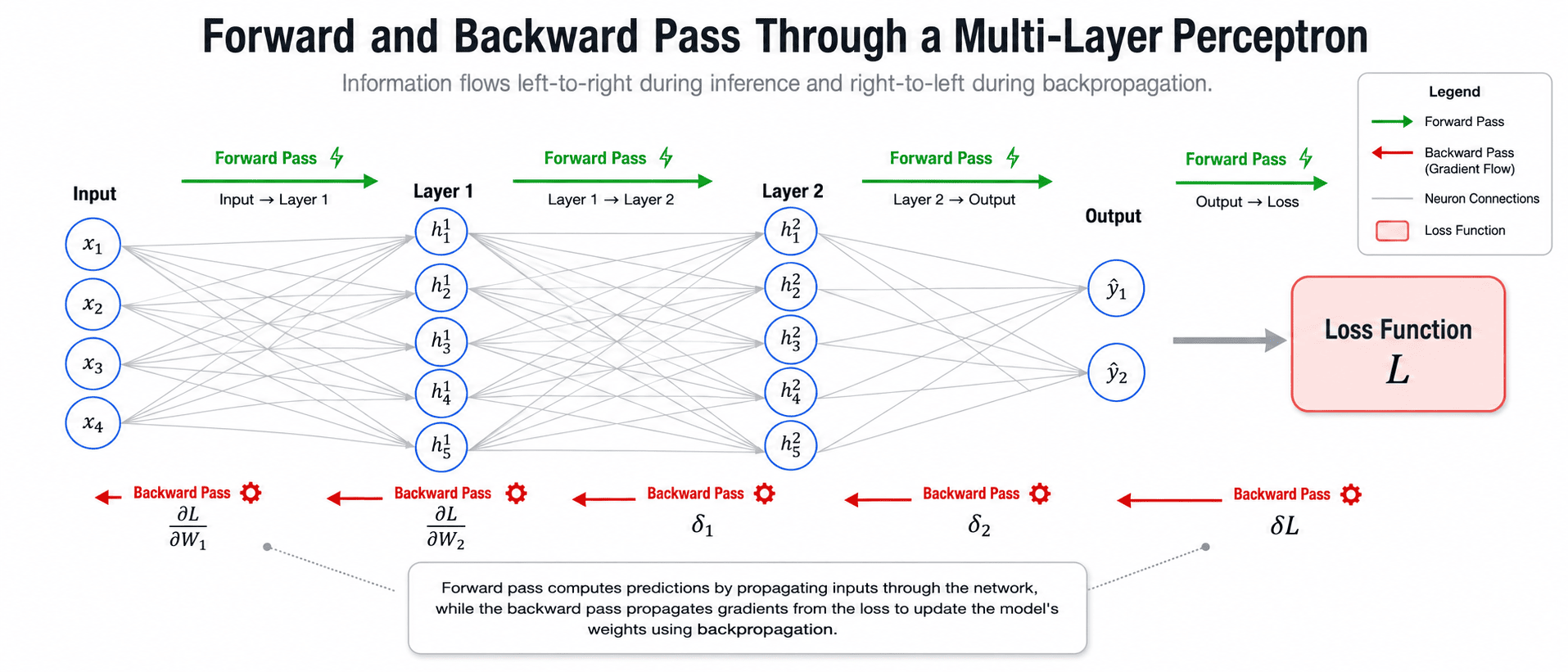
যেকোনো ফর্মুলা দেখার আগেই এই ছবিটি মাথায় গেঁথে নিন:
- ফরওয়ার্ড পাস (Forward pass): তথ্য বাম থেকে ডানে প্রবাহিত হয় — ইনপুট → লেয়ার ১ → লেয়ার ২ → ... → আউটপুট → লস।
- ব্যাকওয়ার্ড পাস (Backward pass): দোষ বা ভুলের দায় ডান থেকে বামে প্রবাহিত হয় — লস → আউটপুট লেয়ার → ... → লেয়ার ২ → লেয়ার ১।
- প্রতিটি লেয়ারে, ব্যাকপ্রোপাগেশন একটি মূল জিনিস ক্যালকুলেট করে: এই লেয়ারের raw আউটপুটে খুব সামান্য পরিবর্তন আনলে চূড়ান্ত লস কতটা বদলে যাবে? এই সংবেদনশীলতা বা সেনসিটিভিটিকেই বলা হয় ওই লেয়ারের এরর সিগন্যাল (error signal), যাকে লেখা হয় দিয়ে।
- একবার আপনি কোনো লেয়ারের এরর সিগন্যাল জেনে গেলে, ওই লেয়ারের ওয়েট গ্রেডিয়েন্টগুলো বের করা শুধুই সাধারণ পাটিগণিত — তখন আর ক্যালকুলাসের কোনো কাজ বাকি থাকে না। এখানকার সব কঠিন কাজটাই হলো -কে পেছনের দিকে ঠিকমতো প্রবাহিত করা।
ফরওয়ার্ড পাস (Forward pass)
ইনপুট প্রতিটি লেয়ারের ভেতর দিয়ে প্রবাহিত হয়, প্রতি ধাপে z এবং a সেভ বা ক্যাশ (cache) করে রাখে, এবং শেষে একটি প্রেডিকশন ও একটি লস তৈরি করে।
আউটপুট এরর (Output error)
একেবারে শেষের লেয়ারে δ ক্যালকুলেট করা হয়: নেটওয়ার্কের raw আউটপুটের সাপেক্ষে লস কীভাবে রিয়্যাক্ট করে বা রেসপন্স করে।
ব্যাকওয়ার্ড রিকার্শন (Backward recursion)
δ-কে লেয়ারে লেয়ারে পেছনের দিকে প্রবাহিত করা হয়, যেখানে ফরওয়ার্ড পাসের সময় সেভ করে রাখা ওয়েটস এবং অ্যাক্টিভেশনগুলো পুনরায় ব্যবহার করা হয়।
প্যারামিটার গ্রেডিয়েন্টস (Parameter gradients)
প্রতিটি লেয়ারে, δ-কে কংক্রিট বা নির্দিষ্ট ওয়েট এবং বায়াসের গ্রেডিয়েন্টে পরিণত করা হয় — যা গ্রেডিয়েন্ট ডিসেন্টের জন্য একদম প্রস্তুত।
এর পেছনের গণিত (The Math Behind It)
আমরা ফরওয়ার্ড-প্রোপাগেশনের নোটেশনগুলোই আবার ব্যবহার করছি: , , এবং per-example লস যা যেকোনো ডিফারেনশিয়েবল (differentiable) লস ফাংশন হতে পারে।
আউটপুট থেকে শুরু করে পেছনের দিকে ইনপুটে আসার পথে ব্যাকপ্রোপাগেশন প্রতিটি লেয়ারে ঠিক এই একটি জিনিসই ক্যালকুলেট করে। বাকি সবকিছু এখান থেকেই বেরিয়ে আসে।
কম্পিউটেশন গ্রাফ হিসেবে একটি নেটওয়ার্ক (A Network as a Computational Graph)
চেইন রুল প্রয়োগ করার আগে, এটি কল্পনা করা সাহায্য করে যে একটি নেটওয়ার্ক আসলে একটি কম্পিউটেশন গ্রাফ (computational graph) — অর্থাৎ ছোট ছোট, সহজ অপারেশনের (গুণ, যোগ, নন-লিনিয়ারিটি) একটি চেইন, যেখানে প্রতিটি নোড শুধু তার ঠিক আগের নোডগুলোর ওপর নির্ভর করে। ফরওয়ার্ড পাসে, ইনপুট এই গ্রাফের প্রতিটি নোড দিয়ে একবার করে পার হয়ে একটি সংখ্যা তৈরি করে (লস)। ব্যাকওয়ার্ড পাসে, আমরা প্রশ্ন করি: "যদি এই নোডের আউটপুট সামান্য বদলে যায়, তবে একদম শেষের লসটি কতটা বদলাবে?" — আর চেইন রুল আমাদের বলে দেয় যে এই প্রশ্নের উত্তর পাওয়ার জন্য শুধু প্রতিবেশী নোডগুলোর লোকাল ডেরিভেটিভগুলো গুণ করে যেতে হবে।
এই দৃষ্টিভঙ্গিটি গুরুত্বপূর্ণ কারণ এটি দেখায় যে ব্যাকপ্রোপাগেশন কোনো নিউরাল নেটওয়ার্ক-নির্দিষ্ট ট্রিক নয় — এটি যেকোনো ডিফারেনশিয়েবল কম্পিউটেশন গ্রাফের জন্য কাজ করে। একটি MLP-তে গ্রাফটি খুব নিয়মিত (প্রতিটি লেয়ার একই প্যাটার্ন পুনরাবৃত্তি করে), কিন্তু একই মূলনীতি যেকোনো জটিল, শাখা-প্রশাখাযুক্ত গ্রাফের জন্যও প্রযোজ্য — এটাই হলো আধুনিক অটোগ্রাড (autograd) ইঞ্জিনগুলোর ভিত্তি।
ধাপ ১ — আউটপুট লেয়ারের এরর (Step 1 — The Output Layer Error)
চেইন রুল অনুসারে, একেবারে শেষ লেয়ার -এর এররটি দুটি উপাদানে ভাগ হয়ে যায়:
যেখানে: হলো নেটওয়ার্কের raw আউটপুটের সাপেক্ষে লসের গ্রেডিয়েন্ট, আর হলো এলিমেন্ট-ওয়াইজ (Hadamard) গুণফল, কারণ অ্যাক্টিভেশন ফাংশনটিও এলিমেন্ট-ওয়াইজ বা উপাদান-ভিত্তিতে প্রয়োগ করা হয়।
পেছনের যুক্তি বা Intuition: এই এররটি মূলত প্রেডিকশনটি কতটা ভুল তার সাথে অ্যাক্টিভেশন ফাংশনটি ওই মুহূর্তে কতটা সেনসিটিভ বা সংবেদনশীল, এই দুটোর মিশ্রণ। একটি খাড়া অ্যাক্টিভেশন ঢালের (steep activation slope) সাথে একটি বড় লস গ্রেডিয়েন্ট মিলে একটি বড় এরর সিগন্যাল তৈরি করে — আর এদের যেকোনো একটি শূন্যের কাছাকাছি হলে পুরো সিগন্যালটিও ছোট হয়ে যায়।
একটি খুব বিখ্যাত সিম্প্লিফিকেশন (A famous simplification)
খুব পরিচিত দুটি জোড়ার ক্ষেত্রে — বাইনারি ক্রস-এন্ট্রপির সাথে সিগময়েড অ্যাক্টিভেশন, এবং ক্যাটাগরিক্যাল ক্রস-এন্ট্রপির সাথে সফটম্যাক্স — এই পুরো এক্সপ্রেশন বা রাশিটি ভেঙে খুব সহজ একটি রূপে পরিণত হয়: । চ্যাপ্টার ১৬-তে এটি খুব স্পষ্টভাবে প্রতিপাদন করা হয়েছে; এটি Deep Learning-এ সবচেয়ে বেশি পরীক্ষা করা বা টেস্ট করা রেজাল্টগুলোর একটি, কারণ এটি খুব পরিষ্কার: গ্রেডিয়েন্ট হলো শুধুই প্রেডিকশন থেকে আসল টার্গেট বিয়োগ করার ফল।
ব্যাকওয়ার্ড রিকার্শন এবং ভ্যানিশিং গ্রেডিয়েন্টের যোগসূত্র (How the Recursion Connects to Vanishing Gradients)
ব্যাকওয়ার্ড রিকার্শনের সমীকরণটি লক্ষ করলেই বোঝা যায় কেন গভীর নেটওয়ার্কগুলো ভ্যানিশিং গ্রেডিয়েন্ট সমস্যায় ভোগে: প্রতিটি লেয়ার পেছনে যাওয়ার সময় -কে এবং দিয়ে গুণ করা হয়। যদি একটি -লেয়ারের নেটওয়ার্কে প্রতিটি -এর মান ধারাবাহিকভাবে ছোট থাকে (যেমন সিগময়েডের সর্বোচ্চ মান মাত্র ), তবে আউটপুট থেকে ইনপুট পর্যন্ত পৌঁছাতে -কে প্রায় বার এরকম ছোট সংখ্যা দিয়ে গুণ করা হয় — ফলে এরর সিগন্যালটি এক্সপোনেনশিয়ালি ছোট হয়ে যায় (-এর ক্রম অনুসারে)। এই একই মেকানিজম উল্টো দিক থেকেও ঘটতে পারে: যদি ওয়েট এবং ডেরিভেটিভগুলো ধারাবাহিকভাবে বড় থাকে, তবে গ্রেডিয়েন্ট এক্সপোনেনশিয়ালি বেড়ে ফেটে পড়তে পারে (এক্সপ্লোডিং গ্রেডিয়েন্ট)।
এই পর্যবেক্ষণটিই পরের চ্যাপ্টারের (অ্যাক্টিভেশন ফাংশন) মূল প্রেরণা: ReLU-এর মতো ফাংশন বেছে নেওয়া হয় আংশিকভাবে ঠিক এই কারণেই — কারণ পজিটিভ ইনপুটের জন্য এর ডেরিভেটিভ হুবহু , যা এই বারবার গুণ হওয়ার প্রক্রিয়ায় সিগন্যালকে সংকুচিত হতে দেয় না।
ধাপ ২ — এরর-কে পেছনের দিকে প্রবাহিত করা (Step 2 — Propagating the Error Backward)
এটাই হলো অ্যালগরিদমটির প্রাণ: লেয়ার -এর এরর-কে তার ঠিক সামনের লেয়ারের এরর-এর সাথে সম্পর্কিত করা।
এটি যেখান থেকে আসে: লেয়ার -এর প্রি-অ্যাক্টিভেশন শুধুমাত্র লেয়ার -এর ভেতর দিয়ে লসকে প্রভাবিত করে। একটি নির্দিষ্ট নিউরন লেয়ার -এর যে যে নিউরনে ইনপুট দেয়, তার প্রতিটির ওপর যোগফল বা সামেশন নিলে (multivariate chain rule অনুযায়ী) পাওয়া যায়:
যাকে একসাথে প্রতিটি নিউরন -এর জন্য লিখলে, ঠিক ওপরের ওই ম্যাট্রিক্স রিকার্শনটিই (matrix recursion) পাওয়া যায়।
কেন 'ব্যাক'-প্রোপাগেশন? (Why 'back'-propagation?)
-কে ক্যালকুলেট করতে আপনার -কে দরকার, যার আবার -কে দরকার, আর এভাবেই চলতে থাকে — একেবারে আউটপুট পর্যন্ত। এই নির্ভরশীলতার বা ডিপেন্ডেন্সির শেকলের কারণেই এরর সিগন্যালগুলো একেবারে আউটপুট থেকে শুরু করে পেছনের দিকে ক্যালকুলেট করা হয়, যা ঠিক ফরওয়ার্ড পাসের আয়নার প্রতিবিম্বের মতো।
ধাপ ৩ — এরর সিগন্যালগুলোকে গ্রেডিয়েন্টে পরিণত করা (Step 3 — Turning Error Signals Into Gradients)
একবার প্রতিটি জানা হয়ে গেলে, আসল ট্রেইন করার মতো বা trainable প্যারামিটারগুলো সরাসরি বেরিয়ে আসে — আর কোনো চেইন রুলের দরকার হয় না।
প্রতিপাদনের একটি রূপরেখা: যেহেতু , তাই আমরা পাই এবং । চেইন রুল প্রয়োগ করে একে ম্যাট্রিক্স আকারে লিখলে ওপরের আউটার প্রোডাক্টটি (outer product) পাওয়া যায়।
হাতে-কলমে গাণিতিক উদাহরণ: ২-লেয়ার নেটওয়ার্কে ব্যাকপ্রোপাগেশন (Worked Example: Backpropagation Through a 2-Layer Network)
আমরা চ্যাপ্টার ১৩-এর উদাহরণটিকে সামনে টেনে আনছি: ইনপুট , সব জায়গায় সিগময়েড অ্যাক্টিভেশন, এবং ফরওয়ার্ড পাস আগেই ক্যালকুলেট করা আছে যেখানে , , , এবং । আসল লেবেল বা টার্গেট হলো , এবং আমরা সিগময়েড আউটপুটের সাথে বাইনারি ক্রস-এন্ট্রপি ব্যবহার করছি — তাই ওপরের সেই সিম্প্লিফিকেশনটি ব্যবহার করে:
লেয়ার ২-এর গ্রেডিয়েন্টগুলো:
ব্যবহার করে, লেয়ার ১-এ ব্যাকওয়ার্ড রিকার্শন:
লেয়ার ১-এর গ্রেডিয়েন্টগুলো:
গ্রেডিয়েন্ট ডিসেন্টের এক ধাপ ফেলার জন্য দরকারি সব গ্রেডিয়েন্ট এখন হাতের মুঠোয় — যা শুধুমাত্র ওই লেয়ারের লোকাল জিনিসপত্র এবং একটিমাত্র ব্যাকওয়ার্ড পাসের মাধ্যমেই ক্যালকুলেট করা হয়েছে।
এই ফিল্ডের সবচেয়ে বেশি জিজ্ঞাসিত ডেরিভেশন প্রশ্ন (The most-asked derivation question in the field)
ইন্টারভিউগুলোতে Deep Learning-এর সবচেয়ে পরিচিত প্রশ্ন সম্ভবত "ব্যাকপ্রোপাগেশনের ডেরিভেশন দেখাও"। স্মৃতি থেকে এগুলো হুবহু লিখতে পারার জন্য তৈরি থাকুন: (১) -এর সংজ্ঞা, (২) আউটপুট লেয়ারের ফর্মুলা, (৩) ব্যাকওয়ার্ড রিকার্শন এবং এর চেইন-রুল ডেরিভেশন, এবং (৪) ওয়েট/বায়াস গ্রেডিয়েন্টের ফর্মুলাগুলো। ওপরের ওই নিউমেরিক উদাহরণটি না দেখে নিজে নিজে প্র্যাকটিস করাটা খুব দারুণ একটা উপায়।
দ্বিতীয় হাতে-কলমে উদাহরণ: গ্রেডিয়েন্ট ডিসেন্টের একটি সম্পূর্ণ আপডেট ধাপ (A Second Worked Example: One Full Gradient Descent Update)
শুধু গ্রেডিয়েন্ট ক্যালকুলেট করে থেমে না গিয়ে, চলুন সেগুলো ব্যবহার করে ওয়েটগুলো আসলেই আপডেট করে দেখি — অর্থাৎ ব্যাকপ্রোপাগেশন এবং গ্রেডিয়েন্ট ডিসেন্টের (gradient descent) মধ্যে সংযোগটি সম্পূর্ণ করি। ওপরের ক্যালকুলেট করা গ্রেডিয়েন্টগুলো ব্যবহার করে, লার্নিং রেট দিয়ে একটি ধাপ ফেলি:
একইভাবে লেয়ার ১-এর ওয়েটগুলোও আপডেট হবে: । এই নতুন ওয়েটগুলো দিয়ে যদি আবার ফরওয়ার্ড পাস চালানো হয়, তবে দেখা যাবে আগের থেকে বেড়ে টার্গেট -এর দিকে সামান্য এগিয়ে গেছে — ঠিক এভাবেই, ছোট ছোট ধাপে ধাপে, লক্ষ লক্ষ বার পুনরাবৃত্তি করে একটি নেটওয়ার্ক ধীরে ধীরে ট্রেন হতে থাকে।
প্রতিটি আপডেট কেন এত ছোট রাখা হয়
লার্নিং রেট ইচ্ছাকৃতভাবে ছোট রাখা হয় (এখানে ব্যবহৃত আসলে তুলনামূলকভাবে বড়, শুধু হাতে-কলমে হিসাবটি স্পষ্ট দেখানোর জন্য) কারণ গ্রেডিয়েন্ট শুধু বর্তমান বিন্দুতে লস কমার দিকটি নির্দেশ করে — অনেক বড় একটি লাফ দিলে সহজেই ওই লোকাল অনুমানটি ভেঙে পড়তে পারে এবং লস আসলে বেড়েও যেতে পারে। লার্নিং রেট নির্বাচনের খুঁটিনাটি অপ্টিমাইজেশন চ্যাপ্টারে বিস্তারিত আলোচনা করা হয়েছে।
Implementation
python
sigmoid_deriv-এর ভেতরের কমেন্টটি বা মন্তব্যটি দেখতে যত সাধারণ মনে হচ্ছে, এটি আসলে তার চেয়েও বেশি গুরুত্বপূর্ণ: এই ফাংশনটি raw প্রি-অ্যাক্টিভেশন নেয় না, বরং এটি নেয় অ্যাক্টিভেশন , কারণ -কে আগে থেকেই ক্যালকুলেট করে রাখা -এর সাপেক্ষে সরাসরি লেখা যায়। ঠিক এই কারণেই ফরওয়ার্ড পাসের সময় প্রতিটি এবং সেভ করে বা ক্যাশ (cache) করে রাখা হয় — ব্যাকপ্রোপাগেশন সবকিছু নতুন করে ক্যালকুলেট না করে শুধু এগুলোকেই পুনরায় ব্যবহার করে।
ব্যাকপ্রোপাগেশনের খরচ প্রায় ফরওয়ার্ড পাসের সমান (Backpropagation is nearly as cheap as the forward pass)
সাধারণভাবে মনে হতে পারে যে মিলিয়ন মিলিয়ন প্যারামিটারের গ্রেডিয়েন্ট ক্যালকুলেট করা নিশ্চয়ই একটিমাত্র ফরওয়ার্ড পাসের চেয়ে অনেক বেশি ব্যয়বহুল। কিন্তু বাস্তবে, ব্যাকপ্রোপাগেশনের খরচ শুধু ফরওয়ার্ড পাসের একটি ছোট গুণিতক (constant factor) বেশি হয় — সাধারণত ২-৩ গুণ — কারণ এটি স্ক্র্যাচ থেকে নতুন করে কিছু ক্যালকুলেট করার বদলে ফরওয়ার্ড পাসের সেভ করে রাখা ভ্যালুগুলোকেই কাজে লাগায়। এর বিকল্প হিসেবে যদি আমরা সসীম পার্থক্য বা finite differences-এর সাহায্যে প্রতিটি প্যারামিটারের গ্রেডিয়েন্ট স্বাধীনভাবে অনুমান করার চেষ্টা করতাম, তবে সেই খরচ প্যারামিটারের সংখ্যার সাথে তাল মিলিয়ে বাড়তে থাকত, যা আজকের বিশাল মডেলের যুগে কম্পিউটেশনালভাবে এক কথায় অসম্ভব।
মূল বিষয়গুলো (Key Takeaways)
Key Takeaways
- ব্যাকপ্রোপাগেশন ক্রেডিট অ্যাসাইনমেন্ট সমস্যার সমাধান করে: প্রতিটি লেয়ারের জন্য খুব দক্ষভাবে ক্যালকুলেট করে।
- এরর সিগন্যাল -কে আউটপুট লেয়ার থেকে শুরু করে পেছনের দিকে রিকার্সিভভাবে (recursively) ক্যালকুলেট করা হয়।
- ব্যাকওয়ার্ড রিকার্শনটি সরাসরি মাল্টিভেরিয়েট চেইন রুল থেকে আসে: ।
- একবার জানা হয়ে গেলে, ওয়েট এবং বায়াসের গ্রেডিয়েন্টগুলো এরর সিগন্যালের সাধারণ আউটার প্রোডাক্ট (outer products) বা সরাসরি কপি হয়ে যায়।
- ব্যাকপ্রোপাগেশনের খরচ মোটামুটিভাবে একটি ফরওয়ার্ড পাসের কম্পিউটেশন খরচের সমানই — আর ঠিক এ কারণেই ডিপ নেটওয়ার্ক ট্রেন করা আদৌ সম্ভব হয়েছে।
সাধারণ ভুল ধারণা (Common Mistakes)
δ-কে ওয়েট গ্রেডিয়েন্ট ভেবে ভুল করা
হলো প্রি-অ্যাক্টিভেশনের সাপেক্ষে বের করা একটি গ্রেডিয়েন্ট, ওয়েটের সাপেক্ষে নয়। এটি মূলত মাঝপথের একটি উপাদান — পেতে হলে আপনাকে আরও একটি ধাপ (অর্থাৎ -এর সাথে আউটার প্রোডাক্ট) এগোতে হবে।
ডেরিভেটিভে ভুল ইনপুট ব্যবহার করা
ফর্মুলাটি অ্যাক্টিভেশন -এর সাপেক্ষে লেখা। স্ক্র্যাচ থেকে এটি ইমপ্লিমেন্ট করার সময়, আগে থেকে সেভ করে রাখা অ্যাক্টিভেশন -এর বদলে raw প্রি-অ্যাক্টিভেশন বসিয়ে দেওয়াটা খুব সাধারণ একটি বাগ বা ভুল।
একাধিক লেয়ারে δ পুনরায় ব্যবহার না করে প্রতিটি লেয়ারের জন্য চেইন রুল নতুন করে ডেরাইভ করা
δ^[ℓ] একবার ক্যালকুলেট হয়ে গেলে সেটিকেই পরবর্তী (আগের) লেয়ারের ক্যালকুলেশনের ভিত্তি হিসেবে ব্যবহার করা উচিত — প্রতিটি লেয়ারের জন্য একেবারে গোড়া থেকে লস পর্যন্ত সম্পূর্ণ চেইন রুল নতুন করে লেখা একটি সাধারণ কিন্তু অপ্রয়োজনীয় ভুল, যা রিকার্শনের পুরো বিন্দুটাকেই মিস করে ফেলে এবং হাতে-কলমে ডেরিভেশনে সহজেই ভুল আনার সম্ভাবনা বাড়িয়ে দেয়।
ইন্টারভিউ কর্নার (Interview Corner)
Quick Check
বাস্তবে এটি কোথায় দেখা যায় (Where This Shows Up in Practice)
PyTorch, TensorFlow, JAX-এর মতো প্রতিটি ডিপ লার্নিং ফ্রেমওয়ার্কই মূলত একটি অটোমেটিক ডিফারেনসিয়েশন ইঞ্জিনকে (automatic differentiation engine) ঘিরে তৈরি হয়েছে, আর একটু গভীরে গেলে দেখা যায় যে এই ইঞ্জিনটি মূলত যেকোনো আর্বিট্রারি কম্পিউটেশন গ্রাফের জন্য সাধারণীকৃত বা generalized হওয়া ব্যাকপ্রোপাগেশন ছাড়া আর কিছুই নয়। হাতে-কলমে এই চ্যাপ্টারের ডেরিভেশনটি বুঝতে পারলেই ভ্যানিশিং গ্রেডিয়েন্ট (চ্যাপ্টার ১৫), গ্রেডিয়েন্ট ক্লিপিং, এবং আধুনিক অপ্টিমাইজারের (চ্যাপ্টার ১৭) মতো বিষয়গুলো পরিষ্কার হতে শুরু করে — কারণ এগুলো সবই হলো এরর সিগন্যালের পেছনের দিকে বয়ে চলার এই ধারাটিকে মসৃণ ও সুশৃঙ্খল রাখার এক একটি ভিন্ন কৌশল।