Chapter 8 of 25
The Birth of the Multi-Layer Perceptron
Stacking neurons to escape a straight line
12 min read
Created ২ আগ, ২০২৬
ভূমিকা (Motivation)
আগের চ্যাপ্টারটি আমাদেরকে একটি কাজের রেসিপি বা সমাধান দিয়ে শেষ হয়েছিল — কয়েকটি perceptron-কে লেয়ারের পর লেয়ার সাজালেই আপনি XOR সলভ করতে পারবেন — কিন্তু শুধু একটি নির্দিষ্ট লজিক গেটের রেসিপি কখনো পুরো থিওরি বা তত্ত্ব হতে পারে না। স্বাভাবিকভাবেই এরপর যে বড় প্রশ্নটি আসে তা হলো: লেয়ার সাজিয়ে যদি XOR-কে বাঁচানো যায়, তবে এটি আর কী কী বাঁচাতে পারে? এমন কি কোনো প্রবলেম আছে যা সাজানো perceptron-গুলো এখনো ছুঁতে পারে না, নাকি এই ধারণাটি বিশাল ও জটিল বাস্তব দুনিয়ার যেকোনো প্যাটার্ন পর্যন্ত স্কেল বা কাজ করতে পারে?
১৯৮০-এর দশকের শেষের দিকে এর যে উত্তরটি গাণিতিকভাবে প্রমাণিত হয়েছিল, তা সত্যিই বিস্ময়কর: এভাবে তৈরি করা একটি নেটওয়ার্ক নীতিগতভাবে যেকোনো যুক্তিসঙ্গত বা ওয়েল-বিহেভড (well-behaved) ফাংশনকে অ্যাপ্রক্সিমেট (approximate) করতে পারে, যা আপনি শিখতে চাইতে পারেন। এই একটি মাত্র তাত্ত্বিক প্রমাণের কারণেই এই চ্যাপ্টারের আর্কিটেকচার — অর্থাৎ Multi-Layer Perceptron (MLP) — কেবল শুরুর দিকের Neural Network-এর ভিত্তিই হয়নি, বরং পরবর্তীতে আসা প্রায় প্রতিটি Deep Learning আর্কিটেকচারেরও ভিত্তি হয়ে উঠেছে।
এই দুই ঘটনার (XOR-এর অসম্ভবতা এবং Universal Approximation Theorem) মাঝের সময়টুকু নিয়ে একটু ভাবা দরকার। ১৯৬৯ থেকে ১৯৮৬ সাল পর্যন্ত — প্রায় সতেরো বছর — Minsky ও Papert-এর সমালোচনার প্রভাবে Neural Network গবেষণায় ফান্ডিং প্রায় নাই গিয়েছিল। কিন্তু আর্কিটেকচারের ধারণাটি (লেয়ারের পর লেয়ার সাজানো) পুরোপুরি হারিয়ে যায়নি — Paul Werbos তার ১৯৭৪ সালের PhD থিসিসে backpropagation-এর একটি প্রাথমিক রূপ বর্ণনা করেছিলেন, যদিও তখন এটি মূলধারার মনোযোগ পায়নি। ১৯৮৬ সালে David Rumelhart, Geoffrey Hinton এবং Ronald Williams-এর বিখ্যাত Nature পেপার প্রকাশিত হওয়ার পরই backpropagation ব্যাপকভাবে জনপ্রিয় হয় এবং পুরো ফিল্ডকে নতুন জীবন দেয়। এই ইতিহাসটি মনে রাখা জরুরি, কারণ এটি দেখায় যে একটি ভালো আইডিয়া কখনো কখনো এক দশকেরও বেশি সময় ধরে "চাপা পড়ে" থাকতে পারে, শুধু সঠিক টুলসের (এখানে, একটি দক্ষ ট্রেনিং অ্যালগরিদম) অভাব থাকার কারণে।
একটি বাস্তব জীবনের উদাহরণ (A Real-Life Scenario)
কয়েকটি ফিচারের ওপর ভিত্তি করে একটি বাড়ির দাম প্রেডিক্ট করার কথা ভাবুন: বাড়ির আয়তন (square footage), বেডরুমের সংখ্যা, আশেপাশের এলাকার অপরাধের হার (crime rate), এবং সবচেয়ে কাছের স্কুলটির দূরত্ব। এই ফিচারগুলো এবং দামের মধ্যকার আসল সম্পর্কটা কোনো সরলরেখা নয় — একটি খুব ছোট বাড়িতে হয়তো চার নম্বর বেডরুমটি খুব একটা দাম বাড়াবে না, কিন্তু একটি বড় বাড়িতে এর ভালোই মূল্য থাকতে পারে; আবার কোনো এলাকায় হয়তো অপরাধের হার খুব বড় প্রভাব ফেলে, কিন্তু অন্য কোনো এলাকায় হয়তো সেটার তেমন কোনো প্রভাবই নেই। এগুলোই হলো সেই ফিচার ইন্টারঅ্যাকশন (interactions), যা একটি সিঙ্গেল perceptron কোনোভাবেই রিপ্রেজেন্ট করতে পারে না।
একটি MLP ঠিক এই জায়গাটাতেই কাজ করে; সে নেটওয়ার্কটিকে নিজের মতো করে কিছু মাঝের বা ইন্টারমিডিয়েট (intermediate) কনসেপ্ট তৈরি করার জায়গা দেয়। একটি হিডেন নিউরন হয়তো "বড় পারিবারিক বাড়ি" চিনতে শিখতে পারে, যা আয়তন এবং বেডরুমের সংখ্যাকে কোনো নন-লিনিয়ার উপায়ে মেলায়; অন্য একটি নিউরন হয়তো "আকর্ষণীয় এলাকা" চিনতে পারে, যা অপরাধের হার এবং স্কুলের দূরত্বকে মেলায়। এরপর আউটপুট লেয়ারটি এই শেখা কনসেপ্টগুলোকে — যে কনসেপ্টগুলো কেউ হাত দিয়ে ডিজাইন করেনি — একসাথে মিলিয়ে দামের একটি চূড়ান্ত প্রেডিকশন দেয়। একটি perceptron এবং একটি MLP-এর মধ্যে মূল পার্থক্য এটাই: নেটওয়ার্কটি কেবল একটি সরাসরি ইনপুট-থেকে-আউটপুট নিয়ম শেখে না, বরং সে নিজেই নিজের জন্য প্রয়োজনীয় কিছু ইন্টারমিডিয়েট রিপ্রেজেন্টেশন (intermediate representations) বা কনসেপ্ট শিখে নেয়।
মূল ধারণা তৈরি করা (Building the Intuition)
একটি MLP হলো মূলত পর পর যুক্ত থাকা অনেকগুলো perceptron-এর মতো লেয়ার:
- একটি ইনপুট লেয়ার (input layer), যা শুধু raw ফিচারগুলো গ্রহণ করে — এখানে কোনো ক্যালকুলেশন বা গণনা হয় খন, এটি শুধু ডেটা ধরে রাখে।
- এক বা একাধিক হিডেন লেয়ার (hidden layers), যার প্রতিটি তার আগের লেয়ারের সাথে পুরোপুরি যুক্ত (fully connected) থাকে। এখানে প্রতিটি নিউরন তার ইনপুটগুলোর একটি ওয়েটেড সাম (weighted sum) বের করে এবং সেটিকে একটি নন-লিনিয়ার (nonlinear) অ্যাক্টিভেশন ফাংশনের ভেতর দিয়ে পার করে।
- একটি আউটপুট লেয়ার (output layer), যা চূড়ান্ত প্রেডিকশনটি তৈরি করে।
Multi-Layer Perceptron হলো একটি ফিডফরোয়ার্ড (feedforward) আর্টিফিশিয়াল Neural Network, যা একটি ইনপুট লেয়ার, এক বা একাধিক হিডেন লেয়ার এবং একটি আউটপুট লেয়ার নিয়ে গঠিত। এখানে প্রতিটি লেয়ার তার পরের লেয়ারের সাথে পুরোপুরি যুক্ত (fully connected) থাকে, এবং হিডেন বা আউটপুট লেয়ারের প্রতিটি নিউরন তার ইনপুটের ওয়েটেড সামের ওপর একটি নন-লিনিয়ার অ্যাক্টিভেশন ফাংশন প্রয়োগ করে। এর প্যারামিটারগুলো (ওয়েট এবং বায়াস) backpropagation অ্যালগরিদম ব্যবহার করে গ্রেডিয়েন্ট-ভিত্তিক অপ্টিমাইজেশনের মাধ্যমে লস ফাংশনকে (loss function) কমানোর বা মিনিমাইজ করার মাধ্যমে শেখা হয়।
সহজ কথায়: "ফিডফরোয়ার্ড" মানে হলো তথ্য কেবল একদিকে প্রবাহিত হয় — ইনপুট থেকে আউটপুটের দিকে, কোনো লুপ বা পেঁচানো পথ থাকে না। "ফুলি কানেক্টেড" (বা "ডেন্স / dense") মানে হলো এক লেয়ারের প্রতিটি নিউরন তার আগের লেয়ারের প্রতিটি নিউরনের আউটপুট দেখতে পায়। আর নন-লিনিয়ার অ্যাক্টিভেশন ফাংশনটি হলো সবচেয়ে গুরুত্বপূর্ণ উপাদান — এটি ছাড়া লেয়ারের পর লেয়ার সাজালে গাণিতিকভাবে তা মিলে গিয়ে শুধু একটি সিঙ্গেল লিনিয়ার লেয়ারেই পরিণত হবে, আর আমরা আবার সেই perceptron-এর সীমাবদ্ধতাতেই ফিরে যাব।
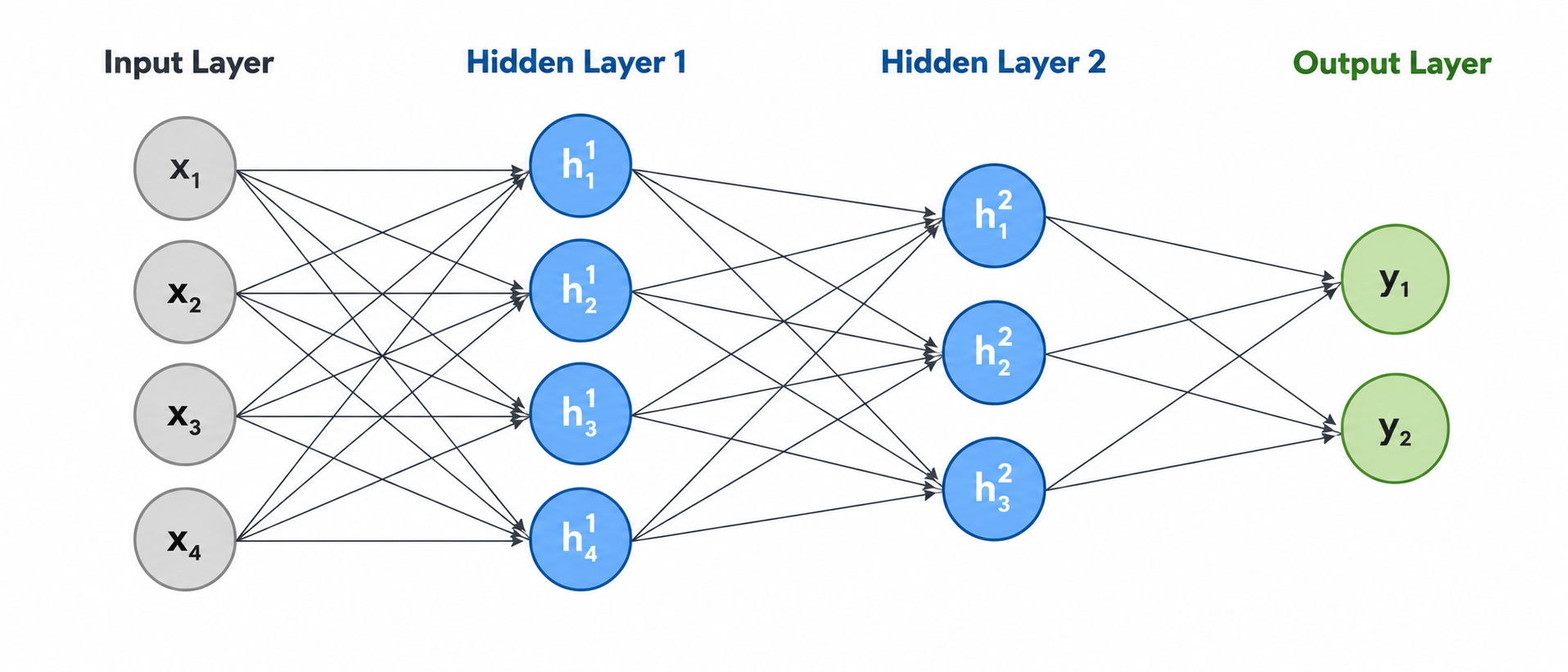
সামনের চ্যাপ্টারগুলোতে আমরা এই ডায়াগ্রামের প্রতিটি অংশ — ওয়েট, বায়াস, অ্যাক্টিভেশন ফাংশন এবং কীভাবে তথ্য সামনের দিকে যায় আর এরর (error) সিগন্যালগুলো পেছনের দিকে আসে — তা নিয়ে অত্যন্ত বিস্তারিত আলোচনা করব। এই চ্যাপ্টারের কাজ হলো শুধু বড় ছবিটি (big picture) দেখানো এবং সেই সাথে সবচেয়ে গুরুত্বপূর্ণ তাত্ত্বিক প্রমাণটি তুলে ধরা, যা বুঝিয়ে দেয় কেন এই আর্কিটেকচারটির এত গভীরে যাওয়াটা সার্থক।
কেন প্রতিটি লেয়ারকে "ফুলি কানেক্টেড" হতে হবে (Why Every Layer Must Be Fully Connected)
একটি স্বাভাবিক প্রশ্ন উঠতে পারে: প্রতিটি নিউরনকে আগের লেয়ারের প্রতিটি নিউরনের সাথে যুক্ত করার দরকার কী? কেন শুধু কিছু নির্বাচিত কানেকশন রাখা হয় না? উত্তরটি হলো নমনীয়তা (flexibility): ট্রেনিং শুরুর আগে আমরা জানি না ঠিক কোন ইনপুট কম্বিনেশনগুলো প্রেডিকশনের জন্য গুরুত্বপূর্ণ হবে। ফুলি কানেক্টেড আর্কিটেকচার নেটওয়ার্ককেই এই সিদ্ধান্ত নেওয়ার স্বাধীনতা দেয় — ট্রেনিংয়ের সময় গুরুত্বহীন কানেকশনগুলোর ওয়েট প্রায় শূন্যের কাছাকাছি চলে যায়, কার্যত সেগুলোকে "নিষ্ক্রিয়" করে দেয়, অথচ প্রয়োজনীয় কানেকশনগুলো শক্তিশালী থেকে যায়। এই সাধারণ (generic) কাঠামোর একটি মূল্যও আছে অবশ্য: এটি অনেক বেশি প্যারামিটার তৈরি করে, যা পরবর্তী চ্যাপ্টারগুলোতে (যেমন Overfitting এবং Regularization) আলোচিত সমস্যাগুলোর জন্ম দেয়। এই ট্রেড-অফটি মনে রাখা ভালো: CNN-এর মতো আর্কিটেকচার (এই কোর্সের পরবর্তী অংশে) স্থানিক (spatial) ডেটার জন্য ইচ্ছাকৃতভাবে কম কানেক্টেড কাঠামো ব্যবহার করে, ঠিক এই ট্রেড-অফটিকেই ভিন্নভাবে সমাধান করার জন্য।
এর পেছনের গণিত: ইউনিভার্সাল অ্যাপ্রক্সিমেশন থিওরেম (The Math Behind It: The Universal Approximation Theorem)
ধরি, হলো একটি নন-কনস্ট্যান্ট, বাউন্ডেড (bounded) এবং কন্টিনিউয়াস (continuous) অ্যাক্টিভেশন ফাংশন। তাহলে একটি সিঙ্গেল হিডেন লেয়ার বিশিষ্ট ফিডফরোয়ার্ড নেটওয়ার্ক, যেখানে অ্যাক্টিভেশন ব্যবহার করা নির্দিষ্ট (কিন্তু সম্ভবত অনেক বড়) সংখ্যক নিউরন রয়েছে, সেটি -এর একটি কমপ্যাক্ট সাবসেটে (compact subset) যেকোনো কন্টিনিউয়াস ফাংশনকে আপনার কাঙ্ক্ষিত যেকোনো পরিমাণ নির্ভুলতার সাথে অ্যাপ্রক্সিমেট (approximate) করতে পারবে — যদি তাকে পর্যাপ্ত পরিমাণ হিডেন ইউনিট বা নিউরন দেওয়া হয়।
সহজ কথায়: যদি আপনার কাছে পর্যাপ্ত সংখ্যক "বাঁকা" (bent) বিল্ডিং ব্লক থাকে (প্রতিটি হিডেন নিউরন পুরো ফাংশনটিতে একটি মসৃণ বাঁক যোগ করে), তবে আপনি মোটামুটি যেকোনো মসৃণ কার্ভ (curve) বা পৃষ্ঠতল (surface) তৈরি করতে পারবেন। ঠিক যেমন অনেকগুলো ছোট ছোট সোজা রেখা দিয়ে যেকোনো কার্ভ তৈরি করা যায়, যদি আপনি যথেষ্ট সংখ্যক রেখা ব্যবহার করেন।
১৯৮৯ সালে এটি স্বাধীনভাবে প্রমাণিত হয়েছিল — সিগময়েড (sigmoid) অ্যাক্টিভেশনের জন্য George Cybenko দ্বারা, এবং আরও সাধারণ ক্ষেত্রে Kurt Hornik, Maxwell Stinchcombe এবং Halbert White দ্বারা। এই থিওরেমটিই হলো সেই গাণিতিক কারণ যার জন্য MLPs-কে এমন সব প্রবলেম সলভ করার জন্য বিশ্বাস করা হয়, যা আগে থেকে কোনো মানুষ বিশ্লেষণ করেনি।
কোনো কিছুর অস্তিত্ব থাকা মানেই সেটার সমাধান হাতে পাওয়া নয়
এই থিওরেমটিকে ভুল বোঝার সম্ভাবনা খুব বেশি, এবং Deep Learning-এ এটি সবচেয়ে সাধারণ ভুলগুলোর একটি। এই থিওরেম শুধু গ্যারান্টি দেয় যে একটি উপযুক্ত নেটওয়ার্কের অস্তিত্ব আছে। এটি আপনাকে কখনোই বলে না:
- আপনার আসলে কতগুলো হিডেন ইউনিট দরকার — একটি সিঙ্গেল হিডেন লেয়ারের জন্য এই সংখ্যাটা অকল্পনীয় রকম বড় হতে পারে, আর ঠিক একারণেই ব্যবহারিক ক্ষেত্রে বিশাল চওড়া (width) লেয়ারের বদলে গভীরতা (depth) ব্যবহার করা হয়।
- কীভাবে সঠিক ওয়েটগুলো খুঁজে বের করতে হবে — gradient descent সত্যি সত্যিই সেই ওয়েটগুলো খুঁজে পাবে কি না, সে বিষয়ে থিওরেমটি কিছুই বলে না।
- নেটওয়ার্কটি নতুন ডেটায় জেনারালাইজ (generalize) করবে কি না — নাকি এটি শুধু তাকে যে উদাহরণগুলো দেখানো হয়েছে সেগুলোকেই মুখস্থ করবে, তা নিয়ে এর কোনো গ্যারান্টি নেই।
রিপ্রেজেন্টেশনাল ক্যাপাসিটি (Representational capacity), ট্রেইনেবিলিটি (trainability) এবং জেনারালাইজেশন (generalization) হলো সম্পূর্ণ আলাদা তিনটি বিষয়। এদেরকে গুলিয়ে ফেলাটা এই ফিল্ডের সবচেয়ে বেশি হওয়া কনসেপচুয়াল ভুলগুলোর একটি।
একটি ক্লাসিক ইন্টারভিউ প্রশ্ন
"যদি একটি সিঙ্গেল হিডেন লেয়ার তাত্ত্বিকভাবে যেকোনো ফাংশনকে অ্যাপ্রক্সিমেট করার জন্য যথেষ্ট হয়, তবে আমরা কেন অনেক লেয়ার বিশিষ্ট ডিপ (deep) নেটওয়ার্ক ব্যবহার করি?" এর একটি মজবুত উত্তরে তিনটি পয়েন্ট থাকা উচিত: (১) একটি সিঙ্গেল চওড়া হিডেন লেয়ার দিয়ে কাঙ্ক্ষিত নির্ভুলতা অর্জন করতে হলে একটি ডিপ নেটওয়ার্কের তুলনায় বহুগুণ বেশি (exponentially larger) নিউরনের প্রয়োজন হতে পারে, কারণ গভীরতা নেটওয়ার্কটিকে শুধু চওড়া করার বদলে বিভিন্ন লেয়ারে সহজ ফাংশনগুলোকে জোড়া লাগানোর সুযোগ দেয়; (২) ডিপ নেটওয়ার্কগুলো এমন কিছু রিপ্রেজেন্টেশন শেখে যা হায়ারার্কিক্যাল (hierarchical) এবং পুনরায় ব্যবহারযোগ্য — শুরুর দিকের লেয়ারগুলো সহজ ফিচারগুলো শেখে, আর পরের দিকের লেয়ারগুলো সেগুলোকে মিলিয়ে জটিল ফিচার তৈরি করে; (৩) বাস্তবে, gradient-based অপ্টিমাইজেশন খুব চওড়া ও অগভীর (shallow) নেটওয়ার্কের চেয়ে মোটামুটি গভীর নেটওয়ার্কগুলোতে ভালো সমাধান খুঁজে পায়।
Cybenko বনাম Hornik-Stinchcombe-White: পার্থক্যটা কী?
১৯৮৯ সালে দুটি স্বাধীন প্রমাণ প্রায় একই সময়ে প্রকাশিত হয়েছিল। George Cybenko-র প্রমাণটি নির্দিষ্টভাবে sigmoid-এর মতো "স্কুইশিং" অ্যাক্টিভেশন ফাংশনের জন্য প্রযোজ্য ছিল। Hornik, Stinchcombe এবং White কিছুদিন পরেই একটি আরও সাধারণ সংস্করণ প্রমাণ করেন, যা প্রায় যেকোনো নন-কনস্ট্যান্ট, বাউন্ডেড, কন্টিনিউয়াস অ্যাক্টিভেশন ফাংশনের জন্য প্রযোজ্য। ইন্টারভিউতে এই দুটি নামই উল্লেখ করার প্রয়োজন সাধারণত হয় না, কিন্তু জানা থাকলে ভালো: থিওরেমটি একটি একক গবেষণা নয়, বরং প্রায় একই সময়ে স্বাধীনভাবে একাধিকবার প্রমাণিত একটি ফলাফল, যা এর গুরুত্বকেই তুলে ধরে।
এই থিওরেমের কারণেই MLP-কে প্রায়ই universal function approximator বলা হয়: যদি একে যথেষ্ট বড় একটি আর্কিটেকচার এবং পর্যাপ্ত ট্রেনিং ডেটা দেওয়া হয়, তবে এটি নীতিগতভাবে যেকোনো ইনপুট-আউটপুট ম্যাপিং শিখতে পারে। আর ঠিক এই কারণেই MLP-স্টাইলের ফুলি কানেক্টেড লেয়ারগুলো সব জায়গাতেই দেখা যায় — ট্যাবুলার ডেটার জন্য একটি আলাদা বা স্ট্যান্ড-অ্যালোন (standalone) মডেল হিসেবে, এবং কনভোল্যুশনাল নেটওয়ার্ক বা ট্রান্সফরমারের (Transformers) মতো আরও অনেক জটিল আর্কিটেকচারের ভেতরে লুকানো বিল্ডিং ব্লক হিসেবে।
যে দুটি হারিয়ে যাওয়া জিনিস MLPs-কে ব্যবহারিক রূপ দিয়েছিল (The Two Missing Pieces That Made MLPs Practical)
১৯৮০-এর দশকের শেষভাগেই আর্কিটেকচার এবং এর তাত্ত্বিক প্রমাণ মূলত বোঝা হয়ে গিয়েছিল। কিন্তু একটি MLP তাত্ত্বিকভাবে কাজ করতে পারে এটি জানা, আর তাকে বাস্তবে ট্রেন করতে পারাটা এক জিনিস নয়। তখনো দুটি ব্যবহারিক উপাদান অনুপস্থিত ছিল:
সমস্যা: কীভাবে দোষ বা ক্রেডিট দেওয়া হবে (how to assign blame)
অনেকগুলো লেয়ার জুড়ে থাকা সম্ভাব্য মিলিয়ন মিলিয়ন ওয়েটের মধ্যে, আপনি কীভাবে জানবেন যে চূড়ান্ত ভুলে (final error) ঠিক কোন ওয়েটটি কতটা অবদান রেখেছে?
হারিয়ে যাওয়া টুকরো ১: একটি দক্ষ ট্রেনিং অ্যালগরিদম
Backpropagation (১৯৮৬) চেইন রুল (chain rule) ব্যবহার করে খুব দক্ষতার সাথে প্রতিটি লেয়ারের প্রতিটি ওয়েটের সাপেক্ষে লস-এর (loss) গ্রেডিয়েন্ট হিসাব করে — এটি নিয়ে কোর্সের পরের দিকে একটি আলাদা চ্যাপ্টার রয়েছে।
হারিয়ে যাওয়া টুকরো ২: ডিফারেনশিয়েবল অ্যাক্টিভেশন (differentiable activations)
Perceptron-এর স্টেপ ফাংশনের প্রায় সব জায়গায় গ্রেডিয়েন্ট শূন্য থাকে, তাই এটি ট্রেনিংয়ের জন্য কোনো কাজের সিগন্যাল দিতে পারে না। সিগময়েড (sigmoid) এবং ট্যানএইচ (tanh) (এবং পরে ReLU)-এর মতো মসৃণ ফাংশনগুলো গ্রেডিয়েন্টকে নেটওয়ার্কের ভেতর দিয়ে প্রবাহিত হওয়ার সুযোগ করে দেয়।
ফলাফল: ট্রেনযোগ্য ডিপ নেটওয়ার্ক
এই দুটি জিনিস একসাথে থাকার কারণে, gradient descent নিখুঁত ও দক্ষতার সাথে হিসাব করা গ্রেডিয়েন্টের নির্দেশনায় প্রতিটি লেয়ারের প্রতিটি ওয়েটকে অ্যাডজাস্ট করতে পারে।
কেন স্টেপ ফাংশনকে বিদায় নিতে হয়েছিল
অরিজিনাল perceptron-এ ব্যবহৃত স্টেপ অ্যাক্টিভেশনটি হঠাৎ করে 0 থেকে 1-এ লাফ দেয়, ঠিক ডিসিশন বাউন্ডারিতে এটি নন-ডিফারেনশিয়েবল (non-differentiable), এবং অন্য সব জায়গায় এর ডেরিভেটিভ (derivative) বা গ্রেডিয়েন্ট শূন্য। Gradient descent-এর জন্য একটি শূন্য নয় এমন বা নন-জিরো (nonzero) ডেরিভেটিভ দরকার হয়, যাতে সে বুঝতে পারে ওয়েটটিকে কোন দিকে ধাক্কা দিতে হবে — সব জায়গায় শূন্য থাকা একটি গ্রেডিয়েন্ট আসলে কোনো তথ্যই দেয় না। এই কারণেই আধুনিক MLPs-এর ভেতরে ব্যবহৃত প্রতিটি অ্যাক্টিভেশন ফাংশন মসৃণ এবং ডিফারেনশিয়েবল হয়; আমরা পরের চ্যাপ্টারেই এগুলো নিয়ে বিস্তারিত পড়ব।
গভীরতা বনাম প্রস্থ: একটি সংক্ষিপ্ত উদাহরণ (Depth vs. Width: A Brief Illustration)
গভীরতা কেন এত কার্যকর, তা একটি ছোট উপমা দিয়ে বোঝা যায়। ধরুন আপনাকে "একটি মানুষের মুখ চিনতে হবে" এই কাজটি শেখাতে হবে। একটি অগভীর (shallow) কিন্তু অত্যন্ত চওড়া নেটওয়ার্ককে কল্পনা করুন যাকে প্রতিটি সম্ভাব্য মুখের প্যাটার্ন আলাদা আলাদাভাবে মুখস্থ করতে হয় — কোনো পুনঃব্যবহারযোগ্য (reusable) ধারণা ছাড়াই। বিপরীতে, একটি গভীর নেটওয়ার্ক প্রথম লেয়ারে কিনারা (edges) চিনতে শেখে, পরের লেয়ারে সেই কিনারাগুলো জোড়া দিয়ে চোখ-নাক-মুখের মতো অংশ চিনতে শেখে, আর তার পরের লেয়ারে সেই অংশগুলো জোড়া দিয়ে সম্পূর্ণ মুখ চিনতে শেখে। "কিনারা" ধারণাটি একবার শেখা হলে তা হাজারো ভিন্ন মুখ চেনার কাজে পুনরায় ব্যবহার করা যায় — এই পুনঃব্যবহারযোগ্যতাই গভীর নেটওয়ার্ককে চওড়া নেটওয়ার্কের তুলনায় এত বেশি প্যারামিটার-সাশ্রয়ী করে তোলে।
মূল বিষয়গুলো (Key Takeaways)
Key Takeaways
- একটি MLP হলো ফুলি কানেক্টেড লেয়ারের একটি ফিডফরোয়ার্ড নেটওয়ার্ক, যেখানে নন-লিনিয়ার অ্যাক্টিভেশন ফাংশন থাকে এবং যা backpropagation দিয়ে শুরু থেকে শেষ পর্যন্ত ট্রেন করা হয়। - Universal Approximation Theorem গ্যারান্টি দেয় যে, একটি সিঙ্গেল-হিডেন-লেয়ার MLP-ও নীতিগতভাবে একটি কমপ্যাক্ট ডোমেইনে যেকোনো কন্টিনিউয়াস ফাংশনকে অ্যাপ্রক্সিমেট করতে পারে, যদি তাকে পর্যাপ্ত হিডেন ইউনিট দেওয়া হয়। - এই থিওরেমটি শুধুই রিপ্রেজেন্টেশনাল ক্যাপাসিটি নিয়ে কথা বলে — এটি নতুন ডেটায় জেনারালাইজ করা বা ট্রেনিংয়ের সাফল্য নিয়ে কিছুই বলে না। - বাস্তবে বিশাল চওড়া লেয়ারের বদলে গভীরতাকে বা ডেপথ (depth)-কে বেশি গুরুত্ব দেওয়া হয়, কারণ এটি সাধারণত অনেক বেশি প্যারামিটার-সাশ্রয়ী (parameter-efficient) এবং এটি হায়ারার্কিক্যাল ও পুনরায় ব্যবহারযোগ্য ফিচার শিখতে সাহায্য করে। - Backpropagation এবং ডিফারেনশিয়েবল অ্যাক্টিভেশন ফাংশন — এই দুটিই ছিল সেই হারিয়ে যাওয়া ব্যবহারিক উপাদান, যা MLP-কে একটি তাত্ত্বিক কৌতূহল থেকে একটি ট্রেনযোগ্য ও কার্যকরী আর্কিটেকচারে পরিণত করেছিল।
সাধারণ ভুল ধারণা (Common Mistakes)
Universal Approximation Theorem-কে ট্রেনিংয়ের গ্যারান্টি হিসেবে ধরা
শিক্ষার্থীরা প্রায়ই এই থিওরেমটিকে এমনভাবে উল্লেখ করে যেন এটি ট্রেনিং সফল হওয়ার গ্যারান্টি দেয়। এটি তা করে না — এটি শুধু গ্যারান্টি দেয় যে ওয়েটগুলোর সমস্ত সম্ভাব্য বিন্যাসের মধ্যে কোথাও না কোথাও সঠিক ওয়েটগুলোর অস্তিত্ব আছে। সেই ওয়েটগুলোকে খুঁজে বের করাটা সম্পূর্ণ আলাদা এবং অনেক বেশি কঠিন একটি কাজ, যা gradient descent কেবল কাছাকাছিভাবে সমাধান করতে পারে।
ধরে নেওয়া যে চওড়া হওয়া সবসময় গভীর হওয়ার চেয়ে ভালো
যেহেতু একটি সিঙ্গেল হিডেন লেয়ার তাত্ত্বিকভাবে যথেষ্ট, তাই এটা ভাবা খুব স্বাভাবিক যে শুধু চওড়া হওয়াই আসল কথা। বাস্তবে, একটি অত্যন্ত চওড়া লেয়ার দিয়ে কাঙ্ক্ষিত নির্ভুলতা অর্জন করতে যা নিউরন (এবং ডেটা, ও কম্পিউট) লাগে, তা একটি মোটামুটি গভীর নেটওয়ার্কের চেয়ে বহুগুণ বেশি হতে পারে, কারণ গভীর নেটওয়ার্কগুলো লেয়ারের পর লেয়ার সহজ ফিচারগুলোকে পুনরায় ব্যবহার করতে পারে।
ভাবা যে একটি MLP-তে যত বেশি হিডেন লেয়ার, ততই ভালো
Universal Approximation Theorem-এর ভুল প্রয়োগে অনেকে ধরে নেয় "গভীরতা যত বাড়বে, পারফরম্যান্স তত বাড়বে," যা সবসময় সত্যি নয়। খুব বেশি গভীর নেটওয়ার্ক vanishing/exploding gradient-এর মতো নতুন সমস্যায় ভুগতে পারে (যা পরের কয়েকটি চ্যাপ্টারে আলোচিত হবে), এবং অতিরিক্ত ক্যাপাসিটি প্রায়ই ওভারফিটিংয়ের (overfitting) ঝুঁকি বাড়ায়। "যথেষ্ট গভীরতা" খুঁজে বের করা একটি ব্যবহারিক, পরীক্ষামূলক (empirical) প্রক্রিয়া, কোনো একমুখী নিয়ম নয়।
ইন্টারভিউ কর্নার (Interview Corner)
Quick Check
বাস্তবে এটি কোথায় দেখা যায় (Where This Shows Up in Practice)
আজকাল প্রোডাকশনে থাকা প্রায় প্রতিটি Deep Learning আর্কিটেকচারের ভেতরে ফুলি কানেক্টেড MLP লেয়ারগুলো হলো ডিফল্ট বিল্ডিং ব্লক — ট্রান্সফরমারের (Transformers) ফিডফরোয়ার্ড সাবলেয়ার থেকে শুরু করে কনভোল্যুশনাল নেটওয়ার্কের চূড়ান্ত ক্লাসিফিকেশন হেড পর্যন্ত সব জায়গায় এদের দেখা যায়। আমরা backpropagation প্রমাণ করার আগে এবং একটি MLP-এর মধ্য দিয়ে তথ্য কীভাবে প্রবাহিত হয় তা নিখুঁতভাবে বোঝার আগে, আমাদের দুটি গাণিতিক টুলকিট প্রয়োজন: লিনিয়ার অ্যালজেব্রা (linear algebra), যা ব্যাখ্যা করে কীভাবে পুরো লেয়ারগুলো ডেটাকে একসাথে ট্রান্সফর্ম করে, এবং ক্যালকুলাস (calculus), যা ব্যাখ্যা করে কীভাবে গ্রেডিয়েন্টগুলো এর মধ্য দিয়ে পেছনের দিকে প্রবাহিত হয়। আর ঠিক এগুলো নিয়েই আমাদের পরের দুটি চ্যাপ্টার।