Chapter 10 of 25
Calculus for Neural Networks
Derivatives, gradients, and the chain rule that makes learning possible
19 min read
Created ২ আগ, ২০২৬
ভূমিকা (Motivation)
আগের চ্যাপ্টারের লিনিয়ার অ্যালজেব্রা আপনাকে বলে যে একটি Neural Network কী ক্যালকুলেট করে — অর্থাৎ ম্যাট্রিক্স মাল্টিপ্লিকেশন এবং অ্যাক্টিভেশনের একটি চেইন। আর ক্যালকুলাস (Calculus) হলো সেই জিনিস যা নেটওয়ার্কটিকে বলে দেয় যে সে কীভাবে আরও ভালো হতে পারে। ট্রেনিংয়ের সময় হওয়া প্রতিটি ওয়েট আপডেটের গভীরে আসলে একটি ডেরিভেটিভ (derivative) ক্যালকুলেশন লুকিয়ে থাকে। লিনিয়ার অ্যালজেব্রা যদি নেটওয়ার্কের অ্যানাটমি বা শারীরিক গঠন হয়, তবে ক্যালকুলাস হলো এর শেখার পদ্ধতি বা লার্নিং মেকানিজম।
এই চ্যাপ্টারটি ক্যালকুলাস টুলকিট তৈরি করে — ডেরিভেটিভ, আংশিক ডেরিভেটিভ বা পার্শিয়াল ডেরিভেটিভ (partial derivatives), গ্রেডিয়েন্ট (gradients), এবং সবচেয়ে গুরুত্বপূর্ণ চেইন রুল (chain rule) — যা খুব শিগগিরই আসতে চলা backpropagation-কে পুরোপুরি বোঝার জন্য আপনার প্রয়োজন হবে। চেইন রুল অংশটিকে খুব গুরুত্বের সাথে নিন: কোনো অতিরঞ্জন ছাড়াই বলা যায়, এটি এই পুরো কোর্সের সবচেয়ে গুরুত্বপূর্ণ গাণিতিক অংশ।
একটি বাস্তব জীবনের উদাহরণ (A Real-Life Scenario)
ভাবুন তো, আপনি পাউরুটি বেক করার সময় ওভেনের টেম্পারেচার ডায়াল বা তাপমাত্রার কাঁটা অ্যাডজাস্ট করছেন, যাতে একটি নিখুঁত সোনালি রঙের ক্রাস্ট বা উপরিভাগ পাওয়া যায়। আপনি ডায়ালের পজিশন এবং ক্রাস্টের রঙের মধ্যকার একদম সঠিক ফাংশন বা সম্পর্কটি জানেন না, কিন্তু আপনি পরীক্ষা (experiment) করে দেখতে পারেন: ডায়ালটিকে সামান্য একটু বাড়িয়ে দিন, তারপর দেখুন ক্রাস্টটি আগের চেয়ে দ্রুত নাকি ধীরগতিতে কালো হচ্ছে। এই যে একটু পরিবর্তন করা এবং পর্যবেক্ষণ করার পদ্ধতিটি — অর্থাৎ আমি এই একটি ইনপুটে খুব সামান্য একটু পরিবর্তন করলে আউটপুটে ঠিক কতটা পরিবর্তন হয়? — ঠিক এটাই হলো একটি ডেরিভেটিভের পরিমাপ।
এখন ভাবুন, একটি ডায়ালের বদলে আপনার কাছে এক মিলিয়ন বা দশ লাখ ডায়াল আছে (যা আসলে একটি Neural Network-এর ওয়েট), আর ক্রাস্টের রং চোখের আন্দাজে দেখার বদলে, আপনার কাছে এমন একটি সংখ্যা আছে যা বলে দিচ্ছে পুরো নেটওয়ার্কের প্রেডিকশন কতটা ভুল ছিল (যাকে লস বা loss বলা হয়)। আপনি নিশ্চয়ই এক মিলিয়ন ডায়ালকে একটি একটি করে ঘুরিয়ে দেখতে পারবেন না কী হয় — এতে অনন্তকাল লেগে যাবে। আপনার এমন একটি উপায় দরকার, যা একই সাথে প্রতিটি ডায়ালের জন্য তৎক্ষণাৎ বলে দেবে যে লস কমানোর জন্য কোন ডায়ালটিকে কোন দিকে ঘোরাতে হবে। ঠিক এই কাজটিই গ্রেডিয়েন্ট এবং চেইন রুল করে দেয়, আর ঠিক এ কারণেই এত বড় নেটওয়ার্কের ট্রেনিং আদৌ সম্ভব হয়।
মূল ধারণা তৈরি করা (Building the Intuition)
কোনো সূত্র বা ফর্মুলায় যাওয়ার আগে, এই ধারণাগুলো মাথায় গেঁথে নিন:
- ডেরিভেটিভ (derivative) আপনাকে কোনো ফাংশনের তাৎক্ষণিক পরিবর্তনের হার বা ইনস্ট্যান্টেনিয়াস রেট অফ চেঞ্জ (instantaneous rate of change) বলে দেয় — ইনপুটে খুব সামান্য একটু ধাক্কা দিন, আর ডেরিভেটিভ আপনাকে বলে দেবে আউটপুট ঠিক কতটা এবং কোন দিকে নড়বে।
- পার্শিয়াল ডেরিভেটিভ (partial derivative) ঠিক একই কাজ করে, তবে একসাথে অনেকগুলো চলক বা ভেরিয়েবল থাকা ফাংশনের জন্য। এটি একটি মাত্র ভেরিয়েবল বাদে বাকি সব ভেরিয়েবলকে সাময়িকভাবে স্থির (frozen) হিসেবে ধরে নেয়।
- গ্রেডিয়েন্ট (gradient) প্রতিটি পার্শিয়াল ডেরিভেটিভকে একটি একক ভেক্টরে সংগ্রহ করে, যা ফাংশনটির সবচেয়ে খাড়াভাবে বৃদ্ধির (steepest increase) দিকে নির্দেশ করে — আর এর নেগেটিভটি (negative) ফাংশন কমানোর সবচেয়ে দ্রুত পথের দিকে নির্দেশ করে, যা কোনো লস কমানোর চেষ্টায় আমাদের ঠিক এটাই দরকার হয়।
- চেইন রুল (chain rule) হলো সেই নিয়ম যার মাধ্যমে আপনি একটির ভেতর একটি থাকা ফাংশনের চেইন বা শৃঙ্খলের ভেতর দিয়ে ডেরিভেটিভ ক্যালকুলেট করতে পারেন — আর একটি Neural Network-এ লেয়ারের পর লেয়ার সাজানো থাকা মানেই হলো সেটি একটির ভেতর একটি থাকা ফাংশনের অত্যন্ত দীর্ঘ একটি চেইন ছাড়া আর কিছুই নয়।
এর পেছনের গণিত (The Math Behind It)
ডেরিভেটিভ (The Derivative)
সহজ কথায়: -কে খুব সামান্য একটি পরিমাণ দিয়ে ধাক্কা দিন এবং দেখুন কতটা পরিবর্তিত হয়, তারপর সেই ধাক্কাটিকে শূন্যের কাছাকাছি ছোট করে আনুন। যদি হয়, তবে বাড়ালে বাড়ে; আর যদি হয়, তবে বাড়ালে কমে। ঠিক এই তথ্যটিই ট্রেনিংয়ের সময় কোনো ওয়েটকে কোন দিকে সরাতে হবে সেই সিদ্ধান্ত নিতে ব্যবহার করা হয়: আমরা জানতে চাই যে লস কমানোর জন্য এটিকে কোন দিকে ধাক্কা দিতে হবে।
| ফাংশন (Function) | ডেরিভেটিভ (Derivative) |
|---|---|
| f(x) = c (ধ্রুবক বা constant) | f'(x) = 0 |
| f(x) = xⁿ | f'(x) = nxⁿ⁻¹ |
| f(x) = eˣ | f'(x) = eˣ |
| f(x) = ln(x) | f'(x) = 1/x |
| f(x) = σ(x) = 1/(1+e⁻ˣ) | f'(x) = σ(x)(1−σ(x)) |
| f(x) = tanh(x) | f'(x) = 1 − tanh²(x) |
এই দুটো মুখস্থ করে নিন
একবার যখন আমরা অ্যাক্টিভেশন ফাংশন এবং backpropagation-এ পৌঁছে যাব, তখন ওপরে দেওয়া সিগময়েড এবং ট্যানএইচ-এর ডেরিভেটিভগুলো প্রতিনিয়ত ব্যবহার করা হবে। কোশেন্ট রুল (quotient rule) থেকে অন্তত একবার নিজে নিজে প্রতিপাদন বা ডিরাইভ (derive) করে দেখা বেশ উপকারী, যাতে এটি শুধু মুখস্থ করা কোনো বিষয় হয়ে না থাকে।
পার্শিয়াল ডেরিভেটিভস (Partial Derivatives)
একটি Neural Network-এর লস কেবল একটি ভেরিয়েবলের ওপর নির্ভর করে না — এটি একই সাথে প্রতিটি ওয়েট এবং বায়াসের ওপর নির্ভর করে, যার সংখ্যা মিলিয়ন বা দশ লাখের ঘরে হতে পারে। একসাথে অনেকগুলো ভেরিয়েবল থাকা ফাংশন নিয়ে কাজ করার জন্য আমাদের পার্শিয়াল ডেরিভেটিভ প্রয়োজন হয়।
একটি ফাংশন -এর জন্য, -এর সাপেক্ষে পার্শিয়াল ডেরিভেটিভ, যাকে লেখা হয়, তা নির্দেশ করে যে বাকি সমস্ত ভেরিয়েবল স্থির বা ধ্রুবক রেখে -এর সাপেক্ষে -এর পরিবর্তনের হার কত।
হাতে-কলমে উদাহরণ: ধরি ।
পয়েন্টে: , এবং ।
জ্যামিতিক ছবি: স্পর্শ সমতল (Geometric Picture: The Tangent Plane)
এক-ভেরিয়েবলের ডেরিভেটিভ একটি বক্ররেখার স্পর্শক রেখা (tangent line)-এর ঢাল দেয়; ঠিক একইভাবে, একটি দুই-ভেরিয়েবলের ফাংশনের দুটি পার্শিয়াল ডেরিভেটিভ একসাথে ওই পৃষ্ঠের (surface) একটি নির্দিষ্ট বিন্দুতে স্পর্শ সমতল (tangent plane) বর্ণনা করে। x-অক্ষ বরাবর হাঁটলে পৃষ্ঠটি কতটা খাড়া তা বলে দেয় একটি পার্শিয়াল ডেরিভেটিভ, আর y-অক্ষ বরাবর হাঁটলে কতটা খাড়া তা বলে দেয় অন্যটি, দুটো মিলিয়েই ওই বিন্দুতে পৃষ্ঠের সম্পূর্ণ স্থানীয় ঢাল বা "টিল্ট" ধরা পড়ে।
দ্বিতীয় উদাহরণ — তিনটি ভেরিয়েবল: ধরি g(x,y,z) = x^2yz + 5y।
পয়েন্টে: , , এবং । খেয়াল করুন, প্রতিটি পার্শিয়াল ডেরিভেটিভ নেওয়ার সময় বাকি দুটো ভেরিয়েবলকে সম্পূর্ণ ধ্রুবক ধরা হয়েছে, এমনকি যখন তারা একে অপরের সাথে গুণ আকারে জড়িয়ে আছে (x^2yz-এর মতো), তখনও।
গ্রেডিয়েন্ট (The Gradient)
সহজ কথায়: গ্রেডিয়েন্ট প্রতিটি পার্শিয়াল ডেরিভেটিভকে একটি ভেক্টরে সংগ্রহ করে, যা ওই পয়েন্টে -এর সবচেয়ে খাড়াভাবে বৃদ্ধির (steepest increase) দিকে নির্দেশ করে। এর নেগেটিভ, , সবচেয়ে খাড়াভাবে কমে যাওয়ার দিকে নির্দেশ করে। এই একটি মাত্র ব্যাপারই হলো gradient descent-এর সম্পূর্ণ ভিত্তি: কোনো লস ফাংশন কমাতে চাইলে, প্যারামিটারগুলোকে -এর দিকে সরাতে হয়।
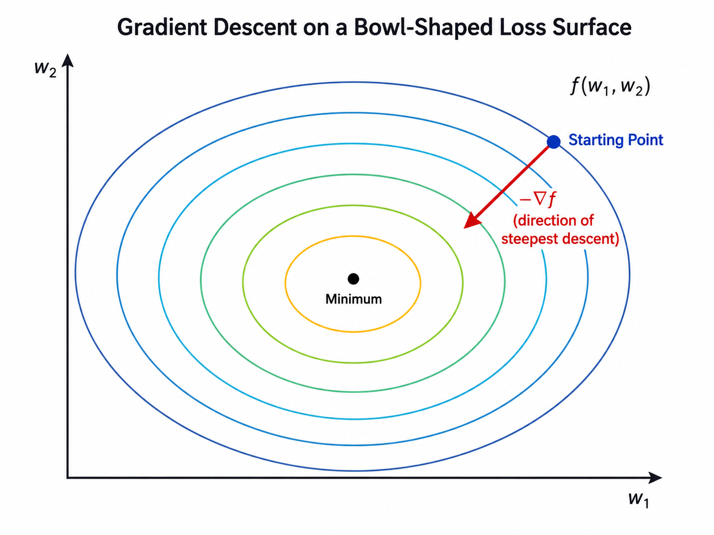
হাতে-কলমে উদাহরণ — গ্রেডিয়েন্ট ক্যালকুলেট করা: ধরি f(x,y) = x^2 + 3y^2। তাহলে গ্রেডিয়েন্ট (2x, 6y)। বিন্দু (1,1)-এ, গ্রেডিয়েন্ট হয় (2,6), এই ভেক্টরটি এমন দিকে নির্দেশ করে যেদিকে f সবচেয়ে দ্রুত বাড়ে। যেহেতু y-এর সহগ (6) x-এর সহগের (2) চেয়ে বড়, তাই ওই বিন্দুতে f, y-দিকের পরিবর্তনে x-দিকের চেয়ে বেশি সংবেদনশীল বা sensitive। gradient descent-এর ক্ষেত্রে প্যারামিটারগুলোকে (-2,-6) দিকে সরানো হবে, অর্থাৎ y-কে x-এর চেয়ে বেশি জোরে টানা হবে, ঠিক কারণ ওই দিকেই লস কমানোর সবচেয়ে বেশি সুযোগ আছে।
দিকনির্দেশক ডেরিভেটিভ (Directional derivative), সংক্ষেপে
গ্রেডিয়েন্ট শুধু "সবচেয়ে খাড়া" দিক বলে দেয় না, এটি যেকোনো দিকে পরিবর্তনের হার হিসাব করতেও ব্যবহার করা যায়। কোনো একক ভেক্টরের দিকে f-এর পরিবর্তনের হার হলো গ্রেডিয়েন্ট এবং ওই একক ভেক্টরের ডট প্রোডাক্ট। এই ডট প্রোডাক্ট তখনই সবচেয়ে বড় হয় যখন একক ভেক্টরটি ঠিক গ্রেডিয়েন্টের দিকেই নির্দেশ করে, এটাই প্রমাণ করে কেন গ্রেডিয়েন্ট আসলেই সবচেয়ে খাড়া বৃদ্ধির দিক নির্দেশ করে।
জ্যাকোবিয়ান এবং হেসিয়ান সম্পর্কে সংক্ষেপে (Jacobians and Hessians, briefly)
যখন একটি ফাংশন স্কেলারের বদলে একটি ভেক্টর আউটপুট দেয় (যেমনটা নেটওয়ার্কের অনেক লেয়ারই করে থাকে), তখন সমস্ত পার্শিয়াল ডেরিভেটিভের সম্পূর্ণ সংগ্রহ একটি ম্যাট্রিক্স তৈরি করে, যাকে জ্যাকোবিয়ান (Jacobian) বলা হয়। যখন আপনি একটি স্কেলার ফাংশনের সেকেন্ড-অর্ডার বা দ্বিতীয় মাত্রার পার্শিয়াল ডেরিভেটিভ নেন, তখন আপনি একটি ম্যাট্রিক্স পান যাকে হেসিয়ান (Hessian) বলা হয়, যা এর স্থানীয় বক্রতা বা কার্ভেচার (curvature) বর্ণনা করে। এই কোর্সের প্রতিপাদনগুলো মূলত ফার্স্ট-অর্ডার বা প্রথম মাত্রার গ্রেডিয়েন্টের ওপর নির্ভরশীল, তবে এই দুটি শব্দ চিনে রাখা ভালো — পুরো লেয়ার জুড়ে একবারে backpropagation বোঝার সময় জ্যাকোবিয়ান স্বাভাবিকভাবেই চলে আসে, আর হেসিয়ান হলো সেকেন্ড-অর্ডার অপ্টিমাইজেশন মেথড এবং লস মিনিমামটি কতটা "ধারালো (sharp)" তার ধারণার মূল ভিত্তি।
চেইন রুল (The Chain Rule)
এটি হলো গণিতের সেই অংশ, যার দিকে এই পুরো কোর্সটি নীরবে এগিয়ে যাচ্ছে। এটি সেই গাণিতিক সত্য যা backpropagation-কে সম্ভব করে তোলে।
যদি এবং হয়, অর্থাৎ যদি -এর ওপর কেবল -এর মাধ্যমেই নির্ভর করে, তবে:
সহজ কথায়: যদি -এর সাপেক্ষে গুণ দ্রুত পরিবর্তিত হয়, এবং -এর সাপেক্ষে গুণ দ্রুত পরিবর্তিত হয়, তবে -এর সাপেক্ষে গুণ দ্রুত পরিবর্তিত হবে। নির্ভরতার একটি চেইন বরাবর পরিবর্তনের হারগুলো কেবল গুণ হতে থাকে।
একটি সাধারণ গাণিতিক উদাহরণ: ধরি । এখানে ধরি, ফলে ।
সরাসরি বিস্তৃত করে বা এক্সপান্ড করে মিলিয়ে দেখুন: , সুতরাং — দুটি পদ্ধতিই একই রেজাল্ট দিচ্ছে, ঠিক যেমনটা তাদের দেওয়ার কথা। নির্দিষ্টভাবে বলতে গেলে, -এর ক্ষেত্রে: , তাই , এবং সরাসরি এক্সপান্ড করলে পাওয়া যায় , যা মিলে যাচ্ছে।
এখন ভাবুন, একটি Neural Network-এ একসাথে অনেকগুলো ভেরিয়েবল অনেকগুলো পথ বা পাথ (paths) দিয়ে চূড়ান্ত লস-এর সাথে যুক্ত হচ্ছে — প্রতিটি বাস্তব লেয়ারেই ঠিক এমনটা ঘটে।
যদি , -এর ওপর নির্ভর করে এবং প্রতিটি যদি -এর ওপর নির্ভর করে, তবে:
এটি কেন গুরুত্বপূর্ণ: একটি MLP-তে, লস একটি শুরুর দিকের লেয়ারের ওয়েট -এর ওপর কেবল পরোক্ষভাবে (indirectly) নির্ভর করে, যা নির্ভর করে ওই ওয়েটের আউটপুটটি পরবর্তীতে যে যে নিউরনকে প্রভাবিত করে তাদের সবার মাধ্যমে। এই মাল্টিভেরিয়েট চেইন রুলই ঠিক সেই জিনিস, যা আমাদের ওই পথগুলোর প্রতিটির অবদানকে যোগ করে ক্যালকুলেট করার সুযোগ দেয় — খুব আক্ষরিক অর্থেই, backpropagation ঠিক এটাই ইমপ্লিমেন্ট করে।
এটিকে একটি কম্পিউটেশনাল গ্রাফ (computational graph) হিসেবে ভাবুন
একটি Neural Network-কে একটি কম্পিউটেশনাল গ্রাফ হিসেবে ভাবুন: একটি ডিরেক্টেড বা নির্দেশিত গ্রাফ যেখানে প্রতিটি নোড হলো একটি অপারেশন (একটি ম্যাট্রিক্স গুণন, একটি যোগ, বা একটি অ্যাক্টিভেশন ফাংশন) এবং এজ বা রেখাগুলো (edges) হলো অপারেশনগুলোর মধ্যে দিয়ে প্রবাহিত হওয়া ডেটা। চেইন রুল বলে: কোনো নোডের সাপেক্ষে চূড়ান্ত লসের ডেরিভেটিভ ক্যালকুলেট করতে হলে, ওই নোড থেকে লস পর্যন্ত যাওয়া প্রতিটি পথের ওপর থাকা স্থানীয় ডেরিভেটিভগুলোকে গুণ করতে হবে, এবং এমন সমস্ত পথের গুণফলগুলোকে যোগ করতে হবে। Backpropagation হলো ঠিক এই কাজটিই নেটওয়ার্কের প্রতিটি প্যারামিটারের জন্য একবারে করার একটি দক্ষ অ্যালগরিদম, যা গ্রাফটিকে ঠিক একবার পেছনের দিকে অতিক্রম করে।
হাতে-কলমে উদাহরণ — একটি টয় নেটওয়ার্কের মধ্য দিয়ে চেইন রুল: ধরি একটি অত্যন্ত ছোট নেটওয়ার্ক আছে: z = wx, a = sigma(z) (সিগময়েড), এবং লস L = (a-y)^2। আমরা dL/dw বের করতে চাই, অর্থাৎ ওয়েট w সামান্য বদলালে লস কতটা বদলায়।
চেইন রুল অনুযায়ী:
ধরি । তাহলে , এবং ।
তাই । এর মানে হলো, w-কে সামান্য বাড়ালে লস সামান্য কমবে (কারণ ডেরিভেটিভ নেগেটিভ)। ঠিক এই সংকেতটাই gradient descent ব্যবহার করে w-কে কোন দিকে আপডেট করতে হবে তা ঠিক করার জন্য। খেয়াল করুন যে এই তিনটি ধাপই, আউটপুট লেয়ারের ডেরিভেটিভ, অ্যাক্টিভেশনের ডেরিভেটিভ, এবং প্রি-অ্যাক্টিভেশনের ডেরিভেটিভ, ঠিক এভাবেই একটি বাস্তব নেটওয়ার্কের প্রতিটি লেয়ারে গুণ হতে হতে পেছনের দিকে প্রবাহিত হয়, যা backpropagation চ্যাপ্টারে সম্পূর্ণ বিস্তারিতভাবে দেখানো হবে।
গ্রেডিয়েন্ট ডিসেন্ট: এক নজরে (Gradient Descent: A First Look)
যেখানে: হলো প্রতিটি ট্রেনযোগ্য বা ট্রেন করা যায় এমন প্যারামিটার (ওয়েট এবং বায়াস), হলো লস, হলো প্যারামিটারগুলোর সাপেক্ষে এর গ্রেডিয়েন্ট, এবং হলো লার্নিং রেট (learning rate)।
সহজ কথায়: যেহেতু সবচেয়ে খাড়াভাবে লস বৃদ্ধির দিকে নির্দেশ করে, তাই এর উল্টো দিকে, অর্থাৎ -এর দিকে পদক্ষেপ নিলে তা কমে। লার্নিং রেট ওই পদক্ষেপের সাইজ বা আকার নিয়ন্ত্রণ করে — ঠিক এই একই আপডেট রুলের ওপর ভিত্তি করেই অপ্টিমাইজেশন (optimization) নিয়ে পরের একটি চ্যাপ্টারে বিস্তারিত আলোচনা করা হয়েছে।
সবসময় ডিফারেনশিয়েবল নয়: ReLU-এর মতো ফাংশন নিয়ে সতর্কতা (A Caveat: Not Everything Is Differentiable Everywhere)
এতক্ষণ যে ফাংশনগুলো নিয়ে কাজ করা হয়েছে (সিগময়েড, ট্যানএইচ, পলিনোমিয়াল) সেগুলো সবখানেই মসৃণ এবং ডিফারেনশিয়েবল। কিন্তু ডিপ লার্নিং-এ সবচেয়ে জনপ্রিয় অ্যাক্টিভেশন ফাংশন, ReLU (), ঠিক বিন্দুতে একটি ধারালো কোণ বা "কিঙ্ক (kink)" তৈরি করে, যেখানে বাম দিক থেকে ঢাল আর ডান দিক থেকে ঢাল । প্রথাগত অর্থে এই বিন্দুতে ডেরিভেটিভটি সংজ্ঞায়িত নয়।
ব্যবহারিক সমাধান (The practical fix)
বাস্তবে এটি কার্যত কোনো সমস্যা তৈরি করে না। ফ্রেমওয়ার্কগুলো x=0-এর জন্য একটি সাবগ্রেডিয়েন্ট (subgradient) বেছে নেয়, সাধারণত 0 অথবা 1, এবং যেহেতু ফ্লোটিং-পয়েন্ট গণনায় ইনপুট ঠিক শূন্য হওয়ার সম্ভাবনা কার্যত শূন্য, তাই এই একক বিন্দুর অনির্ধারিত হওয়া ট্রেনিংয়ের ওপর কোনো লক্ষণীয় প্রভাব ফেলে না। এই ধরনের ফাংশনকে "প্রায় সর্বত্র ডিফারেনশিয়েবল (differentiable almost everywhere)" বলা হয়, আর এটিই deep learning-এ কার্যকর ভিত্তি হিসেবে যথেষ্ট।
কেন এটা গুরুত্বপূর্ণ: শূন্য থেকে backpropagation ইমপ্লিমেন্ট করার সময়, একটি ফাংশনের ডেরিভেটিভ সবজায়গায় "সুন্দরভাবে" সংজ্ঞায়িত থাকবে, এই ধারণা থেকে বেরিয়ে আসা জরুরি। বাস্তব নেটওয়ার্কগুলো এই ধরনের কিঙ্ক বা ধারালো মোড়যুক্ত ফাংশন দিয়ে পরিপূর্ণ (ReLU, Leaky ReLU, max-pooling), আর গ্র্যাডিয়েন্ট ক্যালকুলেশনগুলো এগুলোকে মসৃণভাবেই সামলে নেয়।
Implementation
python
এটি হাতে করা বা ("অ্যানালিটিক্যাল / analytical") ডেরিভেটিভের সাথে খুব ছোট ফাইনাইট ডিফারেন্স (finite differences) ব্যবহার করে বের করা একটি নিউমেরিক্যাল (numerical) অ্যাপ্রক্সিমেশনের তুলনা করে — এখানে -কে সামান্য একটু পরিমাণ দুই দিকেই সরানো হয় এবং এর ফলে -এ কী পরিবর্তন হলো তা মাপা হয়। এই দুটি মান প্রায় হুবহু মিলে যাওয়া উচিত (এখানে দুটোর মানই 42 আসে)। এই পদ্ধতিটিকে গ্রেডিয়েন্ট চেকিং (gradient checking) বলা হয়, এবং আপনি যখন শূন্য থেকে backpropagation ইমপ্লিমেন্ট করবেন, তখন বাগ (bug) ধরার জন্য এটি একটি অমূল্য টুল হিসেবে কাজ করে: এটি এমন সূক্ষ্ম চিহ্নের ভুল বা ভুলভাবে চেইন রুল প্রয়োগ করার ভুল ধরে ফেলে, যা না ধরলে একটি নেটওয়ার্ক নীরবেই ভুলভাবে ট্রেন হতে থাকত।
শূন্য থেকে ইমপ্লিমেন্ট করার সময় বাগ ধরতে গ্রেডিয়েন্ট চেকিং ব্যবহার করুন
যদি আপনার হাতে-করা গ্রেডিয়েন্ট একটি নিউমেরিক্যাল ফাইনাইট-ডিফারেন্স চেকের সাথে দশমিকের পর কয়েক ঘর পর্যন্ত না মেলে, তবে নিউমেরিক্যাল চেকটিকে বিশ্বাস করুন — আপনার অ্যানালিটিক্যাল ডেরিভেটিভ বের করায় বা ইমপ্লিমেন্ট করায় কোথাও একটি বাগ আছে, যা প্রায় সবসময়ই চেইন রুলের কোনো ধাপ ভুল করা বা কোনো প্লাস-মাইনাস চিহ্ন উল্টে যাওয়ার কারণে হয়।
মূল বিষয়গুলো (Key Takeaways)
Key Takeaways
- ডেরিভেটিভ কোনো ফাংশনের তাৎক্ষণিক পরিবর্তনের হার মাপে; আর পার্শিয়াল ডেরিভেটিভ একে একাধিক ভেরিয়েবলের ফাংশনের জন্য সম্প্রসারিত করে, যেখানে বাকি সব ভেরিয়েবলকে স্থির রাখা হয়। - গ্রেডিয়েন্ট প্রতিটি পার্শিয়াল ডেরিভেটিভকে একটি ভেক্টরে সংগ্রহ করে, যা সবচেয়ে খাড়াভাবে বৃদ্ধির দিকে নির্দেশ করে; এর নেগেটিভটি সবচেয়ে খাড়াভাবে কমে যাওয়ার দিকে নির্দেশ করে। - চেইন রুল, , আপনাকে একটির ভেতর একটি থাকা (composed) ফাংশনগুলোর ভেতর দিয়ে ডিফারেনশিয়েট (differentiate) করার সুযোগ দেয় — ঠিক যেমনটা লেয়ার করা Neural Network-এর গঠন হয়ে থাকে। - মাল্টিভেরিয়েট চেইন রুল নির্ভরতার প্রতিটি পথের ওপর থাকা অবদানগুলোকে যোগ করে, এবং এটিই হলো backpropagation-এর নিখুঁত গাণিতিক ভিত্তি। - Gradient descent প্যারামিটারগুলোকে -এর দিকে সরায়, যাকে লার্নিং রেট দিয়ে স্কেল করা হয় বা গুণ করা হয়। - গ্রেডিয়েন্ট চেকিং (অ্যানালিটিক্যাল ডেরিভেটিভের সাথে নিউমেরিক্যাল ফাইনাইট-ডিফারেন্স হিসেবের তুলনা করা) হলো শূন্য থেকে backpropagation ইমপ্লিমেন্ট করার সময় বাগ ধরার একটি সাধারণ উপায়।
সাধারণ ভুল ধারণা (Common Mistakes)
অন্য ভেরিয়েবলগুলোকে ধ্রুবক বা স্থির ধরতে ভুলে যাওয়া
যখন একটি মাল্টিভেরিয়েবল ফাংশনের জন্য ক্যালকুলেট করা হয়, তখন ডিফারেনশিয়েট করার সময় অন্য প্রতিটি ভেরিয়েবলকে অবশ্যই একটি নির্দিষ্ট ধ্রুবক হিসেবে ধরতে হবে — এটি গুলিয়ে ফেলা (ভুল ভেরিয়েবলের সাপেক্ষে ডিফারেনশিয়েট করা, বা কোনো 'ধ্রুবক'-এর ভেতর লুকিয়ে থাকা x-এর ওপর নির্ভরশীল টার্ম ভুলে যাওয়া) হলো পার্শিয়াল ডেরিভেটিভ নিয়ে শুরুর দিকের সবচেয়ে সাধারণ ভুলগুলোর একটি।
চেইন রুলে কোনো একটি চেইন বা লিংক বাদ দিয়ে দেওয়া
যখন কোনো নির্ভরশীলতার চেইনে তিন বা ততোধিক নেস্টেড বা একটার ভেতর একটা ফাংশন থাকে ( নির্ভর করে -এর ওপর, নির্ভর করে -এর ওপর, নির্ভর করে -এর ওপর), তখন ভুল করে একটি লিংক বাদ দিয়ে তিনটির মধ্যে মাত্র দুটি ডেরিভেটিভ একসাথে গুণ করে ফেলার সম্ভাবনা খুব বেশি থাকে। চেইনের প্রতিটি লিংক অবশ্যই অন্তর্ভুক্ত করতে হবে: ।
ডেরিভেটিভ শূন্য মানেই মিনিমাম, এমনটা ধরে নেওয়া
শুধু বলে যে ওই বিন্দুতে ল্যান্ডস্কেপ সমতল, এটি নিশ্চিত করে না যে এটি একটি মিনিমাম। এটি ম্যাক্সিমামও হতে পারে অথবা একটি স্যাডল পয়েন্টও হতে পারে (যেখানে কিছু দিকে বাড়ে, কিছু দিকে কমে)। কোনটা আসলে ঘটছে তা নিশ্চিত করতে সেকেন্ড ডেরিভেটিভ বা হেসিয়ানের দিকে তাকাতে হয়, যা অপ্টিমাইজেশন থিওরি চ্যাপ্টারে বিস্তারিত আলোচনা করা হয়েছে।
নিউমেরিক্যাল ডেরিভেটিভে খুব ছোট বা খুব বড় h বেছে নেওয়া
গ্রেডিয়েন্ট চেকিং করার সময় h অনেক বড় হলে ফাইনাইট-ডিফারেন্স অ্যাপ্রক্সিমেশন ভুল হয়ে যায়, আবার h অনেক ছোট হলে (যেমন 1e-12) ফ্লোটিং-পয়েন্ট রাউন্ডিং এরর প্রাধান্য পেয়ে যায় এবং ফলাফল নয়েজি হয়ে ওঠে। বাস্তবে h এর জন্য প্রায় 1e-5 থেকে 1e-7 এর মধ্যে একটি মান সাধারণত ভালো ভারসাম্য দেয়।
ইন্টারভিউ কর্নার (Interview Corner)
Quick Check
বাস্তবে এটি কোথায় দেখা যায় (Where This Shows Up in Practice)
আজ পর্যন্ত তৈরি হওয়া প্রতিটি Neural Network-এর প্রতিটি ট্রেনিং স্টেপ বা ধাপেই চেইন রুল ব্যবহার করা হয়, যা প্রতিটি লেয়ার জুড়ে স্বয়ংক্রিয়ভাবে এবং দক্ষতার সাথে প্রয়োগ করা হয়, ঠিক ঠিক হিসাব করে যে লস কমানোর জন্য প্রতিটি ওয়েটকে কতটা সরাতে হবে। আগের চ্যাপ্টারের ম্যাট্রিক্স এবং ভেক্টর অপারেশনের সাথে এটি যুক্ত হওয়ার পর, এখন আপনার কাছে backpropagation-কে লেয়ারের পর লেয়ার, চিহ্নের পর চিহ্ন ধরে সম্পূর্ণভাবে প্রতিপাদন করার টুলকিটের দুই অর্ধেকই হাতে চলে এসেছে — আর ঠিক এটি নিয়েই আমাদের এই কোর্সের সামনের আলোচনা, শুধু প্রোবাবিলিটি এবং স্ট্যাটিস্টিকস (probability and statistics) নিয়ে আরেকটি চ্যাপ্টারের পরপরই, যা ব্যাখ্যা করবে কেন আমরা মূলত এই লস ফাংশনগুলোই ব্যবহার করি।