Chapter 23 of 25
MLPs Compared to Other Architectures
When to reach for an MLP, and when not to
15 min read
Created ২ আগ, ২০২৬
ভূমিকা (Motivation)
ডিপ লার্নিংয়ের প্রতিটি আর্কিটেকচার আবিষ্কার হওয়ার পেছনে ঠিক একই কারণ থাকে: কেউ না কেউ এমন একটি দেয়ালে ধাক্কা খেয়েছিল যা তৎকালীন টুলস বা সরঞ্জাম দিয়ে টপকানো সম্ভব ছিল না। যে MLP-র ওপর আপনি এই পুরো কোর্সে দক্ষতা অর্জন করেছেন, সেটি নিজেও এক সময় তেমনই একটি ভেঙে ফেলা দেয়াল ছিল — এটি পারসেপ্ট্রনের নন-লিনিয়ারলি-সেপারেবল (non-linearly-separable) ডেটা সামলাতে না পারার অযোগ্যতা দূর করেছিল। কিন্তু MLP-রও নিজস্ব কিছু দেয়াল বা সীমাবদ্ধতা আছে, এবং এর পরে আসা আর্কিটেকচারগুলো — যেমন CNN, RNN, LSTM, GRU এবং Transformer — প্রতিটিই তৈরি হয়েছে কারণ একটি সাধারণ MLP-কে সরলভাবে বা না ভেবেচিন্তে ব্যবহার করতে গিয়ে মানুষ সরাসরি ওই দেয়ালগুলোর কোনো একটিতে ধাক্কা খেয়েছিল।
এই চ্যাপ্টারটি ওই আর্কিটেকচারগুলো বিস্তারিতভাবে শেখার জন্য নয় (সেটি অন্য কোনো কোর্সের বিষয়)। এটি মূলত এমন একটি প্রশ্নের উত্তর দেওয়ার যোগ্যতা অর্জন করার জন্য যা কেবল ব্যাকপ্রোপাগেশন মুখস্থ করা কাউকে এমন একজন থেকে আলাদা করে যে নিউরাল নেটওয়ার্ককে আসলেই গভীরভাবে বোঝে: একটি নির্দিষ্ট সমস্যা দেওয়া থাকলে, আপনি কেন একটি সাধারণ MLP বেছে নেবেন — অথবা কেন নেবেন না?
একটি বাস্তব জীবনের উদাহরণ (A Real-Life Scenario)
কল্পনা করুন, একই বিকেলে আপনার হাতে সম্পূর্ণ আলাদা তিনটি কাজ দেওয়া হলো। প্রথম কাজ: চল্লিশটি সংখ্যাভিত্তিক কলাম বা ফিচার বিশিষ্ট (যেমন স্কয়ার ফিট, বেডরুমের সংখ্যা, জিপ কোড ইত্যাদি) একটি স্প্রেডশীট বা এক্সেল ফাইল থেকে বাড়ির দাম প্রেডিক্ট বা অনুমান করা। দ্বিতীয় কাজ: একটি ছবির ক্যাপশন লেখা। তৃতীয় কাজ: একটি ইংরেজি বাক্যকে ফরাসিতে অনুবাদ করা।
এই তিনটি কাজের জন্যই হুবহু একই সরঞ্জাম বা টুল ব্যবহার করাটা হবে একটি মস্ত বড় ভুল। স্প্রেডশীটের কাজটি একটি সাধারণ MLP-র জন্য একদম নিখুঁত — কারণ এখানে ডেটা আগে থেকেই অর্থপূর্ণ সংখ্যার একটি নির্দিষ্ট আকারের ভেক্টর (fixed-size vector)। কিন্তু ছবিটির একটি নিজস্ব স্পেশাল বা স্থানিক কাঠামো (spatial structure) আছে যা ছবিটিকে ফ্ল্যাটেন (flatten) বা এক লাইনে সোজা করে ফেললে নষ্ট হয়ে যায়। বাক্যটির দৈর্ঘ্য ও শব্দগুলোর ক্রমানুসার পরিবর্তনশীল, যা একটি ফিক্সড-সাইজ ইনপুট দিয়ে প্রকাশ করা মোটেও সম্ভব নয়। ঠিক কোন কাঠামোগত অমিল বা স্ট্রাকচারাল মিসম্যাচের (structural mismatch) মুখোমুখি আপনি হচ্ছেন তা চেনাটাই আপনাকে একটি গোল ছিদ্রে চারকোনা পেরেক ঠোকার চেষ্টা করার বদলে সঠিক আর্কিটেকচার বেছে নিতে — অথবা ডিজাইন করতে — সাহায্য করবে।
মূল ধারণা তৈরি করা (Building the Intuition)
এখানে একটি মানসিক মডেল বা চিন্তা মাথায় গেঁথে নেওয়া যাক:
- একটি MLP ধরে নেয় যে তার ইনপুটটি হলো স্বাধীন বা ইনডিপেনডেন্ট ফিচারগুলোর একটি নির্দিষ্ট আকারের ভেক্টর (fixed-size vector), যেখানে ইনপুটের একটি পজিশনের সাথে তার পাশের পজিশনের কোনো বিশেষ সম্পর্ক আগে থেকে ধরে নেওয়া হয় না।
- ছবি বা ইমেজ স্থানিক দিক থেকে (spatially) এই ধারণাটি লঙ্ঘন করে — একটি পিক্সেলের চারপাশের প্রতিবেশীদের ভূমিকা অনেক বেশি গুরুত্বপূর্ণ, এবং ছবিটিকে ভেঙে একটি সরল ভেক্টরে রূপান্তর বা ফ্ল্যাটেন করলে সেই গুরুত্বপূর্ণ সম্পর্কটি চিরতরে হারিয়ে যায়।
- সিকোয়েন্সগুলো (টেক্সট, অডিও, টাইম সিরিজ) সময়ের দিক থেকে (temporally) এই ধারণাটি লঙ্ঘন করে — যেমন ৫ নম্বর উপাদানটি নির্ভর করে তার আগে কী এসেছে তার ওপর, এবং এর ইনপুটটির দৈর্ঘ্যও কোনো নির্দিষ্ট বা ফিক্সড আকারের হয় না।
- MLP-র বাইরে তৈরি হওয়া প্রতিটি আর্কিটেকচারকে সবচেয়ে ভালো বোঝার উপায় হলো: "MLP-র সাধারণ-উদ্দেশ্যের মূল যন্ত্রপাতিটি নিন, এবং সেটির সাথে ডেটার ধরনের সাথে মেলে এমন একটি অতিরিক্ত কাঠামোগত অনুমান বা স্ট্রাকচারাল অ্যাজাম্পশন (structural assumption) স্ক্রু দিয়ে জুড়ে দিন।"
এবং সবচেয়ে গুরুত্বপূর্ণ বিষয় হলো — এই নতুন আর্কিটেকচারগুলোর কোনোটিই কিন্তু MLP-কে ফেলে দেয় না। আমরা নিচে যেমনটি দেখব, MLP এদের প্রায় প্রতিটির ভেতরেই বেঁচে থাকে, সাধারণত শেষ লেয়ার বা লেয়ারগুলো হিসেবে যা এক্সট্র্যাক্ট করা ফিচারগুলোকে একটি বাস্তব উত্তরে রূপান্তরিত করে।
MLP-র নিজস্ব চারণভূমি: পারসেপ্ট্রন বনাম MLP (Perceptron vs. MLP)
অন্য কিছুর সাথে MLP-র তুলনা করার আগে, এটি সুনির্দিষ্টভাবে জানা দরকার যে একটি একক পারসেপ্ট্রন থেকে একটি পূর্ণাঙ্গ MLP-তে আপগ্রেড করার মাধ্যমে আমরা বাস্তবে কী পেয়েছি।
| দিক বা Aspect | পারসেপ্ট্রন (Perceptron) | মাল্টি-লেয়ার পারসেপ্ট্রন (MLP) |
|---|---|---|
| লেয়ার বা স্তর | একটিমাত্র লেয়ার | এক বা একাধিক হিডেন লেয়ারের সাথে একটি আউটপুট লেয়ার |
| অ্যাক্টিভেশন | স্টেপ ফাংশন (যা ডিফারেনসিয়েবল নয়) | মসৃণ ও ডিফারেনসিয়েবল নন-লিনিয়ারিটি (ReLU, sigmoid ইত্যাদি) |
| উপস্থাপনযোগ্য ফাংশন | শুধুমাত্র লিনিয়ারলি সেপারেবল ফাংশন | যেই কোনো কন্টিনিউয়াস বা অবিচ্ছিন্ন ফাংশন, যথেষ্ট হিডেন ইউনিট থাকলে (Universal Approximation Theorem) |
| ট্রেনিং অ্যালগরিদম | পারসেপ্ট্রন লার্নিং রুল (এরর-চালিত, কোনো গ্রেডিয়েন্ট নেই) | ব্যাকপ্রোপাগেশন + গ্রেডিয়েন্ট-ভিত্তিক অপ্টিমাইজেশন |
| XOR সমস্যার সমাধান করতে পারে? | না | হ্যাঁ |
MLP বনাম CNN — যখন স্থানিক বা স্পেশাল কাঠামো গুরুত্বপূর্ণ (MLP vs. CNN)
সংক্ষেপে CNN আসলে কী
একটি Convolutional Neural Network (CNN) একটি MLP-র ফুললি-কানেক্টেড লেয়ারগুলোর (কিছু অংশ) জায়গায় কনভোলিউশনাল লেয়ার (convolutional layers) ব্যবহার করে: যা হলো মূলত একটি ছবির স্থানীয় বা লোকাল অঞ্চলগুলোর ওপর দিয়ে স্লাইড করে নিয়ে যাওয়া ছোট ছোট শেয়ারড ফিল্টার (shared filters)। ইনপুট পিক্সেলের প্রতিটি অংশই তার নিজস্ব ইউনিক ওয়েট বা ওজন দিয়ে প্রতিটি নিউরনের সাথে যুক্ত হওয়ার বদলে, প্রতিটি স্থানিক অবস্থানে একই ছোট ওয়েটের সেট বারবার ব্যবহার করা হয়, যা সরাসরি এই বাস্তব সত্যটিকে কাজে লাগায় যে কাছাকাছি থাকা পিক্সেলগুলো পরস্পরের সাথে সম্পর্কিত এবং একটি বিড়ালকে যদি তিন পিক্সেল বাঁয়ে সরিয়ে দেওয়া হয় তবুও সেটি বিড়ালই থাকে।
একটি raw ছবিকে সরাসরি একটি MLP-র ভেতরে পাঠিয়ে দিলে সাথে সাথেই দুটি প্রধান সমস্যা দেখা দেয়। প্রথমত, আপনাকে 2D গ্রিডটিকে ভেঙে একটি 1D ভেক্টরে ফ্ল্যাটেন করতে হবে, যা এই বাস্তব সত্যটি ছুড়ে ফেলে দেয় যে পিক্সেলগুলোর চারপাশের অবস্থান স্থানিক দিক থেকে অত্যন্ত গুরুত্বপূর্ণ — ফ্ল্যাটেন করার পর কাছাকাছি থাকা দুটি পিক্সেল ভেক্টরের ভেতরে হয়তো অনেক দূরে গিয়ে বসতে পারে। দ্বিতীয়ত, প্যারামিটারের সংখ্যা অবাস্তবভাবে লাফিয়ে ওঠে: একটি সাধারণ সাইজের ছবির ওপর একটি ফুললি-কানেক্টেড লেয়ারের জন্য শুধুমাত্র একদম প্রথম লেয়ারেই প্রতি আউটপুট নিউরনে ১,৫০,০০০-এরও বেশি ওয়েট বা ওজনের প্রয়োজন হয়।
| দিক বা Aspect | MLP | CNN |
|---|---|---|
| কানেক্টিভিটি বা সংযোগ | লেয়ারগুলোর মধ্যে ফুললি-কানেক্টেড (সম্পূর্ণ সংযুক্ত) | শেয়ারড কনভোলিউশনাল ফিল্টারের মাধ্যমে লোকালি-কানেক্টেড |
| ছবির জন্য প্যারামিটারের সংখ্যা | প্রচুর (কোনো ওয়েট শেয়ারিং বা অংশীদারিত্ব নেই) | অনেক কম (স্থানিক অবস্থান জুড়ে ওয়েট শেয়ারিং হয়) |
| স্থানিক কাঠামো | সংরক্ষিত থাকে না (ইনপুট ফ্ল্যাটেন করা হয়) | সুনির্দিষ্টভাবে সংরক্ষিত থাকে এবং কাজে লাগানো হয় |
| সাধারণ ব্যবহার | টেবুলার ডেটা, অথবা ফিচার এক্সট্র্যাকশনের পর একটি "হেড" বা মাথা হিসেবে | ছবি এবং অন্যান্য গ্রিড-আকারের ডেটা |
বাস্তব দৃশ্যকল্প: কখন CNN বেছে নেবেন (Worked Scenario: When to Choose a CNN)
যদি আপনার ডেটা এরকম হয় — একগুচ্ছ ছবি, যেখানে একই বস্তু ছবির যেকোনো জায়গায় দেখা যেতে পারে (যেমন একটি বিড়াল ফ্রেমের বাঁয়ে বা ডানে যেকোনো জায়গায় থাকতে পারে) — তাহলে CNN বেছে নিন, কারণ ওয়েট শেয়ারিং একই ফিল্টারকে পুরো ছবি জুড়ে পুনরায় ব্যবহার করতে দেয়, ফলে বস্তুটি কোথায় আছে তা নয়, বরং কী আছে তা শেখা যায়। অন্যদিকে, যদি আপনার ডেটা ইতিমধ্যেই একটি নির্দিষ্ট-অর্থবহ টেবিল হয় (যেমন প্রতিটি কলামের একটি নির্দিষ্ট, স্থির অর্থ আছে — কলাম ৩ সবসময় "বয়স", কলাম ৭ সবসময় "আয়") তাহলে CNN-এর কোনো প্রয়োজন নেই; এই ধরনের ডেটায় কোনো স্থানিক প্রতিসাম্য (spatial symmetry) নেই যা কাজে লাগানো যায়, তাই একটি সাধারণ MLP-ই ভালো এবং সহজ পছন্দ।
MLP বনাম RNN — যখন ক্রমানুসার ও মেমরি গুরুত্বপূর্ণ (MLP vs. RNN)
সংক্ষেপে RNN আসলে কী
একটি MLP একটি নির্দিষ্ট আকারের ইনপুট ভেক্টর আশা করে এবং প্রতিটি ইনপুটকে স্বাধীনভাবে বিচার করে — সেখানে "আগে" বা "পরে" বলে কোনো ধারণা থাকে না। একটি Recurrent Neural Network (RNN) একটি হিডেন স্টেট (hidden state) যুক্ত করে যা প্রতিটি টাইম স্টেপে বা সময়ের ধাপে আপডেট হতে থাকে এবং একটি সিকোয়েন্সের ভেতর দিয়ে তথ্যকে সামনের দিকে বয়ে নিয়ে যায়, যা নেটওয়ার্কটিকে এমন এক ধরনের মেমরি বা স্মৃতির ক্ষমতা দেয় যা একটি MLP-র কাঠামোগতভাবে থাকা অসম্ভব।
ধারাবাহিক বা সিকোয়েন্সিয়াল ডেটার ক্ষেত্রে — যেমন টেক্সট, Time series, অডিও — যেখানে ক্রমানুসার এবং প্রসঙ্গ বা কনটেক্সট (context) পরবর্তী উপাদানের অর্থকে পুরোপুরি বদলে দেয়, সেখানে একটি সাধারণ MLP-র কাছে সেই তথ্য জমা রাখার কোনো জায়গাই থাকে না। "তিন ধাপ আগে কী ঘটেছিল" তা যে "এখন কী ঘটছে"-কে প্রভাবিত করতে পারে, MLP-র কাছে এমন কোনো মেকানিজম বা প্রক্রিয়া নেই।
| দিক বা Aspect | MLP | RNN |
|---|---|---|
| ইনপুট | নির্দিষ্ট আকারের ভেক্টর (Fixed-size vector) | পরিবর্তনশীল দৈর্ঘ্যের সিকোয়েন্স (Variable-length sequence) |
| অতীত ইনপুটের মেমরি বা স্মৃতি | নেই (প্রতিটি ইনপুট স্বাধীনভাবে দেখা হয়) | есть, একটি রিকারেন্ট হিডেন স্টেটের মাধ্যমে |
| ওয়েট শেয়ারিং | বিভিন্ন "অবস্থান" জুড়ে কোনো ওয়েট শেয়ারিং নেই | প্রতিটি টাইম স্টেপে একই ওয়েটস বা ওজন বারবার ব্যবহৃত হয় |
| সাধারণ ব্যবহার | টেবুলার ডেটা | সিকোয়েন্সিয়াল ডেটা (টেক্সট, টাইম সিরিজ, অডিও) |
বাস্তব দৃশ্যকল্প: কখন RNN বেছে নেবেন (Worked Scenario: When to Choose an RNN)
যদি আপনার ডেটা এরকম হয় — একটি ছোট, তুলনামূলক অল্প দৈর্ঘ্যের সিকোয়েন্স (যেমন কয়েকটি সময়ের ধাপ বিশিষ্ট সেন্সর রিডিং, অথবা একটি ছোট বাক্য) যেখানে সাম্প্রতিক অতীতই সবচেয়ে বেশি গুরুত্বপূর্ণ — তাহলে একটি RNN যথেষ্ট হতে পারে, এবং এটি Transformer-এর তুলনায় হালকা ও কম প্যারামিটার বিশিষ্ট। কিন্তু যদি সিকোয়েন্সের শুরুর দিকের তথ্য অনেক পরের ধাপকেও প্রভাবিত করে (long-range dependency), তাহলে সাধারণ RNN দ্রুত ভ্যানিশিং গ্রেডিয়েন্টে ভুগবে — সে ক্ষেত্রে LSTM/GRU বা Transformer-এর দিকে যাওয়াই ভালো।
MLP বনাম LSTM/GRU — যখন দীর্ঘস্থায়ী মেমরি গুরুত্বপূর্ণ (MLP vs. LSTM/GRU)
সংক্ষেপে LSTM এবং GRU আসলে কী
সাধারণ RNN-গুলো অনেকগুলো টাইম স্টেপের পেছনের দিকে ব্যাকপ্রোপাগেট করার সময় মারাত্মকভাবে ভ্যানিশিং গ্রেডিয়েন্ট (vanishing gradient) সমস্যায় ভোগে, যা দীর্ঘস্থায়ী সম্পর্ক বা লং-রেঞ্জ ডিপেন্ডেন্সি শেখা প্রায় অসম্ভব করে তোলে। LSTM (Long Short-Term Memory) এবং GRU (Gated Recurrent Unit) নেটওয়ার্কগুলো এই সমস্যাটির সমাধান করে লার্নেবল বা শিক্ষণীয় গেট (gates) ব্যবহার করে — যা মূলত সিগময়েড-অ্যাক্টিভেটেড ছোট ছোট সুইচ যা নিয়ন্ত্রণ করে হিডেন স্টেটে কোন তথ্য যুক্ত হবে, কোন তথ্য মুছে যাবে, অথবা সেখান থেকে কী পড়া হবে, যা দীর্ঘ সিকোয়েন্স জুড়ে গ্রেডিয়েন্ট প্রবাহকে সচল রাখার জন্য বিশেষভাবে তৈরি করা হয়েছে।
| দিক বা Aspect | MLP | LSTM / GRU |
|---|---|---|
| সিকোয়েন্সিয়াল প্রসেসিং | না | হ্যাঁ |
| লং-রেঞ্জ ডিপেন্ডেন্সি সামলানো | প্রযোজ্য নয় | গেটিং মেকানিজমের (gating mechanisms) মাধ্যমে বিশেষভাবে ডিজাইন করা |
| অভ্যন্তরীণ জটিলতা | সহজ: প্রতি লেয়ারে লিনিয়ার + অ্যাক্টিভেশন | অনেক বেশি জটিল: প্রতি সেলে একাধিক গেট থাকে (LSTM-এ: input, forget, output; GRU-তে: reset, update) |
| MLP-র সাথে সম্পর্ক | প্রযোজ্য নয় | প্রতিটি গেট নিজেই একটি ছোট MLP-র মতো লিনিয়ার-প্লাস-সিগময়েড ট্রান্সফরমেশন |
বাস্তব দৃশ্যকল্প: কখন LSTM/GRU বেছে নেবেন (Worked Scenario: When to Choose LSTM/GRU)
যদি আপনার ডেটা এরকম হয় — মাঝারি দৈর্ঘ্যের সিকোয়েন্স (কয়েক ডজন থেকে কয়েক শত ধাপ) যেখানে দীর্ঘস্থায়ী নির্ভরতা গুরুত্বপূর্ণ, কিন্তু ডেটাসেট এত বড় নয় যে একটি পূর্ণাঙ্গ Transformer ট্রেন করার মতো যথেষ্ট ডেটা বা কম্পিউট সম্পদ আপনার হাতে আছে — তাহলে LSTM/GRU একটি চমৎকার মধ্যম পথ। উদাহরণস্বরূপ, একটি ছোট IoT ডিভাইসের সেন্সর স্ট্রিম থেকে অ্যানোমালি সনাক্ত করা, অথবা সীমিত ভোকাবুলারি বিশিষ্ট টেক্সট শ্রেণীবিন্যাস। যেখানে ডেটা বিপুল পরিমাণে আছে এবং প্যারালাল ট্রেনিং জরুরি, সেখানে Transformer সাধারণত ভালো ফলাফল দেয়।
MLP বনাম Transformer — যখন প্যারালালিজম ও অনেক দীর্ঘ সম্পর্ক গুরুত্বপূর্ণ (MLP vs. Transformer)
সংক্ষেপে Transformer আসলে কী
RNN (এবং LSTM/GRU) একটি সিকোয়েন্সকে একবারে এক ধাপ করে প্রসেস করে, যা বেশ ধীরগতির — পুরো সিকোয়েন্স জুড়ে ট্রেনিংকে প্যারালালাইজ (parallelize) বা সমান্তরাল করা যায় না — এবং অনেক দীর্ঘ সম্পর্কের ক্ষেত্রে এটি এখনও নিখুঁত নয়। Transformers এই রিকারেন্স বা বারবার ফিরে আসার বিষয়টি পুরোপুরি বাদ দেয় এবং এর জায়গায় সেল্ফ-অ্যাটেনশন (self-attention) নিয়ে আসে: এমন একটি মেকানিজম যা একই সাথে একটি সিকোয়েন্সের প্রতিটি জোড়া পজিশনের মধ্যকার সম্পর্ক ক্যালকুলেট করে, যা একই সাথে বিশাল আকারের প্যারালালাইজেশন এবং অনেক বেশি শক্তিশালী লং-রেঞ্জ modeling-এর সুযোগ করে দেয়।
| দিক বা Aspect | MLP | Transformer |
|---|---|---|
| মূল মেকানিজম বা মেথড | ফুললি-কানেক্টেড লিনিয়ার লেয়ার + অ্যাক্টিভেশন | সেল্ফ-অ্যাটেনশন + পজিশন-ওয়াইজ ফিডফরওয়ার্ড (MLP) সাবলেয়ার |
| সিকোয়েন্স জুড়ে প্যারালালাইজ করা | প্রযোজ্য নয় (সিকোয়েন্সের কোনো ধারণা নেই) | সিকোয়েন্সের অবস্থান জুড়ে সম্পূর্ণ প্যারালালাইজ করা সম্ভব |
| লং-রেঞ্জ ডিপেন্ডেন্সি বা দীর্ঘ সম্পর্ক | প্রযোজ্য নয় | ধাপে ধাপে এগোনোর বদলে অ্যাটেনশনের মাধ্যমে সরাসরি সামলানো হয় |
| MLP-র সাথে সম্পর্ক | প্রযোজ্য নয় | প্রতিটি ট্রান্সফর্মার ব্লকের ভেতরে একটি করে MLP সাবলেয়ার থাকে; অ্যাটেনশন নিজে কোনো MLP নয় |
ভিশন ট্রান্সফর্মার (Vision Transformers): ধারণার আরও সাধারণ রূপ
ভিশন ট্রান্সফর্মার (ViT) এই ট্রান্সফর্মার আইডিয়াটি নিয়ে ইমেজের ওপর প্রয়োগ করে: এটি একটি ছবিকে ছোট ছোট নির্দিষ্ট আকারের প্যাচে (patches) ভাগ করে, সেগুলোর প্রতিটিকে লিনিয়ারলি এম্বেড করে (একটি সহজ, কার্যকরভাবে একক-লেয়ারের MLP প্রজেকশন), এবং তৈরি হওয়া সিকোয়েন্স অফ প্যাচ এম্বেডিংসকে একটি স্ট্যান্ডার্ড ট্রান্সফর্মার এনকোডারের ভেতরে পাঠিয়ে দেয় — এখানে কোনো কনভোলিউশনই ব্যবহার করা হয় না। বিশাল ডেটা স্কেলের ক্ষেত্রে, এই সাধারণ-উদ্দেশ্যের সংমিশ্রণটি CNN-কেও হারিয়ে দিতে পারে, যদিও CNN-এর ডিজাইনে স্থানিক গুরুত্ব বা স্পেশাল লোকালিটি "হার্ড-কোড" করা থাকে আর ViT-তে তা থাকে না।
বাস্তব দৃশ্যকল্প: কখন Transformer বেছে নেবেন (Worked Scenario: When to Choose a Transformer)
যদি আপনার ডেটা এরকম হয় — দীর্ঘ সিকোয়েন্স (কয়েকশ থেকে কয়েক হাজার টোকেন), বিপুল পরিমাণ ট্রেনিং ডেটা এবং GPU/TPU-তে বড় আকারে সমান্তরাল ট্রেনিং করার সুযোগ — তাহলে Transformer প্রায় সবসময় সেরা পছন্দ, বিশেষত ভাষা বা দীর্ঘ টাইম-সিরিজের ক্ষেত্রে। তবে ছোট ডেটাসেটে (কয়েক হাজার উদাহরণ) Transformer প্রায়শই ওভারফিট করে ফেলে, কারণ এর সেল্ফ-অ্যাটেনশন মেকানিজমে কোনো ইনডাক্টিভ বায়াস (inductive bias) নেই — এটি ডেটা থেকেই সবকিছু শিখতে হয়। সেক্ষেত্রে একটি ছোট RNN, LSTM, অথবা এমনকি একটি ভালোভাবে ফিচার-ইঞ্জিনিয়ার্ড MLP অনেক বেশি স্থিতিশীল ফলাফল দিতে পারে।
আসল ছবি: একটি সর্বজনীন বিল্ডিং ব্লক হিসেবে MLP (The MLP as a Universal Building Block)
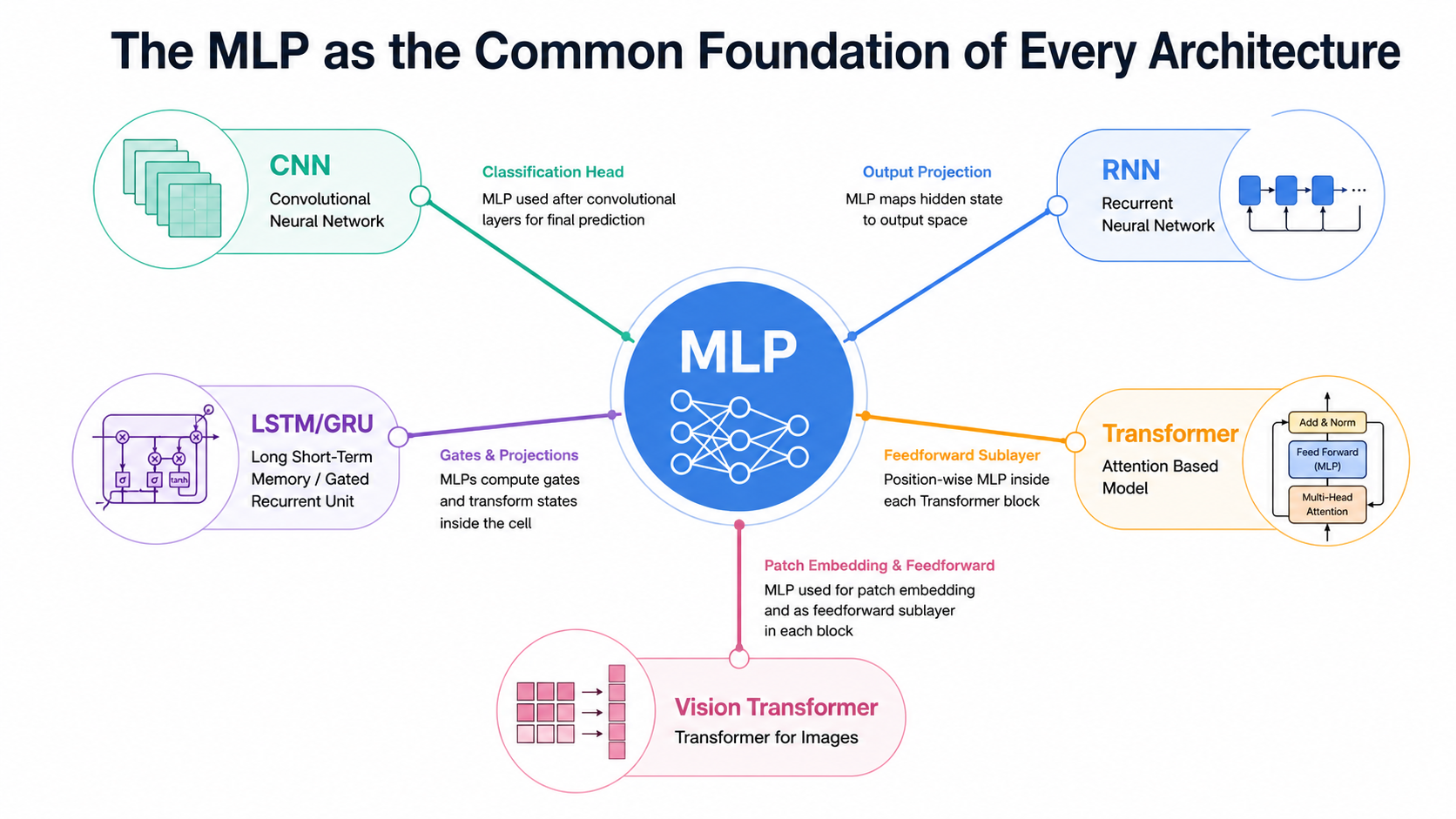
ওপরে তুলনা করা প্রতিটি আর্কিটেকচারের দিকে তাকালে দেখা যাবে, MLP আসলে কখনো হারিয়ে যায় না — এটি বাড়ে একটি গুরুত্বপূর্ণ উপাদান বা কম্পোনেন্ট (component)-এ পরিণত হয়। এটি সাধারণত একদম শেষে যুক্ত করা চূড়ান্ত ক্লাসিফিকেশন বা রিগ্রেশন হেড (classification or regression head) হিসেবে দেখা যায়, অথবা কোনো বিশেষ মেকানিজম (convolution, recurrence, or attention) দ্বারা ডেটার নির্দিষ্ট কাঠামো ক্যাপচার করার কাজ শেষ হওয়ার পর পয়েন্ট-ওয়াইজ নন-লিনিয়ার ট্রান্সফরমেশন হিসেবে কাজ করে।
এই চ্যাপ্টারের সবচেয়ে গুরুত্বপূর্ণ শিক্ষণীয় বিষয় হলো: MLP মূলত CNN, RNN বা Transformers-এর কোনো প্রতিযোগী নয় — এটি বরং এদের সবার সাধারণ ভিত্তি এবং চূড়ান্ত পর্যায়। এই প্রতিটি আর্কিটেকচারই আসলে বাস্তব অর্থে "একটি MLP, যার সাথে নির্দিষ্ট ধরনের কাঠামো সামলানোর জন্য বাড়তি একটি আইডিয়া যুক্ত করা হয়েছে।"
এক নজরে সবার তুলনা (Comprehensive Comparison at a Glance)
| আর্কিটেকচার | যাদের জন্য সবচেয়ে উপযোগী | মূল কাঠামোগত আইডিয়া |
|---|---|---|
| পারসেপ্ট্রন | লিনিয়ারলি সেপারেবল বাইনারি ক্লাসিফিকেশন | একক লিনিয়ার ডিসিশন বাউন্ডারি |
| MLP | টেবুলার ডেটা; সর্বজনীন বিল্ডিং ব্লক | ফুললি-কানেক্টেড লেয়ার + নন-লিনিয়ারিটি |
| CNN | ছবি, গ্রিড-আকারের ডেটা | লোকাল, ওয়েট-শেয়ারড কনভোলিউশনাল ফিল্টার |
| RNN | ছোট সিকোয়েন্স | রিকারেন্ট হিডেন স্টেট (Recurrent hidden state) |
| LSTM / GRU | দীর্ঘতর সিকোয়েন্স | গেটেড রিকারেন্ট হিডেন স্টেট |
| Transformer | দীর্ঘ সিকোয়েন্স, ভাষা বা ল্যাঙ্গুয়েজ, প্যারালালাইজড ট্রেনিং | সেল্ফ-অ্যাটেনশন + MLP সাবলেয়ার |
| Vision Transformer | বড় পরিসরের ছবির কাজ | প্যাচ এম্বেডিং + ট্রান্সফর্মার |
কীভাবে সিদ্ধান্ত নেবেন (A Practical Decision Framework)
একটি নতুন সমস্যার মুখোমুখি হলে নিচের প্রশ্নগুলো ক্রমান্বয়ে নিজেকে জিজ্ঞেস করা একটি দ্রুত এবং কার্যকর উপায়:
১. ইনপুটটি কি একটি ফিক্সড-সাইজ টেবুলার ভেক্টর?
হ্যাঁ হলে, এবং কোনো স্থানিক বা সিকোয়েন্সিয়াল কাঠামো না থাকলে — একটি সাধারণ MLP দিয়েই শুরু করুন। এটি সবচেয়ে সহজ, দ্রুততম এবং প্রায়শই যথেষ্ট।
২. ইনপুটটি কি একটি ছবি বা গ্রিড-আকারের ডেটা?
হ্যাঁ হলে CNN বেছে নিন — স্থানিক লোকালিটি এবং ওয়েট শেয়ারিং আপনাকে অনেক কম প্যারামিটারে ভালো ফলাফল দেবে।
৩. ইনপুটটি কি একটি সিকোয়েন্স, এবং ডেটাসেট ছোট বা মাঝারি?
হ্যাঁ হলে RNN বা LSTM/GRU বিবেচনা করুন, দীর্ঘস্থায়ী নির্ভরতার প্রয়োজন অনুযায়ী।
৪. প্রচুর ডেটা এবং কম্পিউট সম্পদ আছে, দীর্ঘ সিকোয়েন্স নিয়ে কাজ করছেন?
হ্যাঁ হলে Transformer সাধারণত সেরা পারফরম্যান্স দেবে, বিশেষত ভাষাভিত্তিক কাজে।
৫. যেকোনো আর্কিটেকচার বেছে নেওয়ার পরেও
মনে রাখবেন চূড়ান্ত আউটপুট লেয়ার বা হেড হিসেবে প্রায় সবসময়ই একটি MLP ব্যবহৃত হবে — তাই MLP-র জ্ঞান কখনোই অপ্রয়োজনীয় হয় না।
মূল বিষয়গুলো (Key Takeaways)
Key Takeaways
- MLP-র বাইরে তৈরি হওয়া প্রতিটি আর্কিটেকচারই মূলত নির্দিষ্ট ডেটার ধরনের ওপর একটি সাধারণ MLP সরাসরি ব্যবহার করার কাঠামোগত সীমাবদ্ধতা দূর করার জন্য তৈরি হয়েছে: যেমন স্থানিক কাঠামো (CNN), সিকোয়েন্স ও মেমরি (RNN), দীর্ঘস্থায়ী সম্পর্ক (LSTM/GRU), এবং প্যারালালাইজড দীর্ঘস্থায়ী মডেলিং (Transformer)। - CNN স্থানিক লোকালিটি এবং ওয়েট শেয়ারিং কাজে লাগায়; RNN মেমরির জন্য একটি রিকারেন্ট হিডেন স্টেট যোগ করে; LSTM/GRU দীর্ঘ সিকোয়েন্স জুড়ে গ্রেডিয়েন্ট সচল রাখতে গেটিং (gating) ব্যবহার করে; ট্রান্সফর্মার পূর্ণ প্যারালালিটি বা সমান্তরাল কাজের জন্য রিকারেন্স বাদ দিয়ে সেল্ফ-অ্যাটেনশন ব্যবহার করে। - এই সমস্ত বিশেষ মেকানিজম থাকার পরেও, MLP প্রায় প্রতিটির ভেতরেই একটি উপাদান বা কম্পোনেন্ট হিসেবে টিকে থাকে — সবচেয়ে কমনলি চূড়ান্ত আউটপুট হেড হিসেবে, এবং ট্রান্সফর্মারের ক্ষেত্রে প্রতিটি ব্লকের ভেতরে পজিশন-ওয়াইজ ফিডফরওয়ার্ড সাবলেয়ার হিসেবে। - তাই MLP-কে গভীরভাবে বুঝতে পারাটা এই তুলনায় থাকা প্রতিটি আর্কিটেকচারকে ভালোভাবে বোঝার জন্য অত্যন্ত মৌলিক একটি ভিত্তি, এটি এমন কোনো সিঁড়ি নয় যা আপনি এক ধাপ ওঠার পর পেছনে ফেলে চলে যাবেন।
সাধারণ ভুল ধারণা (Common Mistakes)
এই আর্কিটেকচারগুলোকে একে অপরের বিকল্প হিসেবে ধরে নেওয়া
"MLP বনাম CNN বনাম Transformer" কথাটিকে একটি একমুখী পছন্দ হিসেবে ধরে নেওয়া খুব সহজ, যেন একটি সরঞ্জাম বেছে নিলে বাকিগুলো ছুড়ে ফেলতে হবে। বাস্তবে, প্রায় প্রতিটি আধুনিক মডেলই একটি হাইব্রিড বা মিশ্র রূপ — যেমন একটি CNN ব্যাকবোনের সাথে যুক্ত থাকে একটি MLP ক্লাসিফিকেশন হেড, অথবা একটি ট্রান্সফর্মার যার প্রতিটি ব্লকে থাকে একটি করে MLP সাবলেয়ার। প্রশ্নটি প্রায় কখনোই "MLP ব্যবহার করব কি করব না" তা নয়, বরং "MLP-টি ঠিক কোন জায়গায় বসবে এবং কোন বিশেষ মেকানিজমটি একে ইনপুট দেবে" সেটিই মূল বিষয়।
ধরে নেওয়া যে একটি জটিল আর্কিটেকচারই সবসময় সঠিক পছন্দ
CNN, RNN এবং Transformers নির্দিষ্ট কাঠামোগত অমিল দূর করার জন্য তৈরি হয়েছে — এরা সার্বিকভাবে বা সর্বজনীনভাবে MLP-র চেয়ে "সেরা" নয়। কোনো স্থানিক বা সিকোয়েন্সিয়াল কাঠামো না থাকা আসল টেবুলার ডেটার ক্ষেত্রে একটি সাধারণ MLP (অথবা গ্রিডিয়েন্ট-বুস্টেড ট্রির মতো ক্লাসিক্যাল মডেলগুলো) প্রায়শই অনেক বেশি সহজ, উপযুক্ত এবং কম ডেটাতেই অনেক ভালো পারফর্ম করা পছন্দ হতে পারে।
ছোট ডেটাসেটে সরাসরি Transformer বেছে নেওয়া
Transformer-এর সেল্ফ-অ্যাটেনশনে কোনো ইনডাক্টিভ বায়াস (inductive bias) নেই — অর্থাৎ এটি স্থানিক লোকালিটি বা ক্রমানুসারের গুরুত্ব সম্পর্কে আগে থেকে কিছুই ধরে নেয় না, বরং ডেটা থেকেই এসব সম্পর্ক শিখে নিতে হয়। ডেটাসেট ছোট হলে এই নমনীয়তাই কাল হয়ে দাঁড়ায় — মডেলটি সহজেই ওভারফিট করে ফেলে। এমন ক্ষেত্রে CNN, RNN বা এমনকি একটি সাধারণ MLP-ও (যাদের কাঠামোতে ইনডাক্টিভ বায়াস "হার্ড-কোড" করা থাকে) প্রায়ই বেশি স্থিতিশীল ও নির্ভরযোগ্য ফলাফল দেয়।
Interview Corner
Quick Check
বাস্তবে এটি কোথায় দেখা যায় (Where This Shows Up in Practice)
একটি নির্দিষ্ট সমস্যার জন্য কোন কাঠামোগত অনুমানের প্রয়োজন — স্থানিক গুরুত্ব, সিকোয়েন্সিয়াল মেমরি, লং-রেঞ্জ গেটিং, নাকি সম্পূর্ণ প্যারালাল অ্যাটেনশন — তা চিহ্নিত করতে পারার দক্ষতাই মূলত একটি আর্কিটেকচার মুখস্থ করা থেকে সেটিকে সঠিক জায়গায় ব্যবহার করার যোগ্যতাকে আলাদা করে। বাস্তবে, প্রোডাকশনের বেশিরভাগ সিস্টেমই হলো হাইব্রিড বা মিশ্র রূপ: একটি CNN বা Transformer ব্যাকবোন কাঠামো-সচেতন ফিচার এক্সট্র্যাক্ট করে, এবং একটি MLP হেড সেই ফিচারগুলোকে চূড়ান্ত প্রেডিকশনে রূপান্তর করে। এই কোর্সের মতো করে MLP-কে পুঙ্খানুপুঙ্খভাবে জানার অর্থই হলো সেই বড় বড় সিস্টেমগুলোকে একটি ব্ল্যাক বক্স বা রহস্যময় বাক্স হিসেবে না দেখে সেগুলোর প্রতিটি অংশ খুব পরিষ্কারভাবে বুঝতে পারা।