Chapter 9 of 25
Linear Algebra for Neural Networks
Vectors, matrices, and why networks are just matrix math
22 min read
Created ২ আগ, ২০২৬
ভূমিকা (Motivation)
নতুন যারা শিখতে আসেন, তাদের অনেকেই একটা ব্যাপার জেনে অবাক হন: এক মিলিয়ন প্যারামিটার থাকা কোনো Neural Network যখন প্রেডিক্ট করে, তখন সে এক মিলিয়ন আলাদা আলাদা ছোট ছোট ক্যালকুলেশন করে না। সে মূলত খুব অল্প কয়েকটি ম্যাট্রিক্স মাল্টিপ্লিকেশন (matrix multiplications) বা গুণন করে। একটি নিউরনের ভেতরের প্রতিটি ওয়েটেড সাম, এক লেয়ারের সমস্ত নিউরনের একসাথে করা ক্যালকুলেশন, এমনকি ট্রেনিংয়ের সময় পেছনের দিকে প্রবাহিত হওয়া প্রতিটি গ্রেডিয়েন্ট — এই সবকিছুই আসলে লিনিয়ার অ্যালজেব্রা (linear algebra), যাকে Neural Network-এর ভাষায় সাজিয়ে উপস্থাপন করা হয়।
এটি কেবল শোনার জন্য সুন্দর তা-ই নয়, এর একটা খুব ব্যবহারিক গুরুত্বও আছে: লিনিয়ার অ্যালজেব্রার কারণেই Deep Learning এত দ্রুত কাজ করে। GPU-গুলোর একটি বিশেষত্ব হলো এরা খুব দ্রুত বিশাল বিশাল ম্যাট্রিক্স গুণ করতে পারে — আর পুরো Deep Learning সফটওয়্যার স্ট্যাক ঠিক এই সুবিধাটি কাজে লাগানোর জন্যই তৈরি করা হয়েছে। আপনি যদি এই চ্যাপ্টারের অপারেশনগুলো বুঝতে পারেন, তবে কোর্সের বাকি অংশের প্রতিটি সমীকরণ আপনার কাছে আপনার আগে থেকেই জানা পাটিগণিতের মতোই মনে হবে, কোনো অচেনা নোটেশন বা সাংকেতিক চিহ্ন বলে মনে হবে না।
একটি বাস্তব জীবনের উদাহরণ (A Real-Life Scenario)
ভাবুন তো, একটি স্ট্রিমিং সার্ভিস আপনাকে কোনো মুভি সাজেস্ট করার জন্য কীভাবে মূল্যায়ন করে। তারা হয়তো আপনার কয়েকটি ফিচারের ওপর ভিত্তি করে দেখে: আপনি কমেডি কতটা পছন্দ করেন, অ্যাকশন ফিল্ম কতটা পছন্দ করেন, গত পাঁচ বছরে মুভির জন্য আপনার দেওয়া গড় রেটিং কত, ইত্যাদি — ধরুন, এমন মোট ৫০টি ফিচার। এখন ভাবুন, তাদের এই কাজটা শুধু আপনার একার জন্য নয়, বরং প্রতিদিন রাতে ২০,০০০ মুভির বিশাল ক্যাটালগের বিপরীতে ১ কোটি ইউজারের জন্য করতে হয়।
যদি এই গুণটা Python-এর একটি for লুপ ব্যবহার করে একটা একটা করে করা হয়, তবে এটা শেষ হতে অকল্পনীয় সময় লাগবে। কিন্তু এটিকে যদি একটি বিশাল ম্যাট্রিক্স মাল্টিপ্লিকেশন হিসেবে করা হয় — অর্থাৎ প্রতিটি ইউজারের ফিচার ভেক্টরের সাথে প্রতিটি মুভির ফিচার ভেক্টর একেবারে একসাথে গুণ করা হয় — তবে স্পেশালাইজড হার্ডওয়্যার বা GPU-গুলো কয়েক সেকেন্ডের মধ্যেই এই কাজটা শেষ করে ফেলতে পারে। এই চ্যাপ্টারের অপারেশনগুলোই ঠিক এই কাজটি সম্ভব করে তোলে, আর ঠিক এটাই ঘটে একটি MLP-এর প্রতিটি লেয়ারের ভেতর, একটু ছোট স্কেলে।
মূল ধারণা তৈরি করা (Building the Intuition)
নোটেশন বা গাণিতিক চিহ্নে যাওয়ার আগে, এই ধারণাগুলো মাথায় গেঁথে নিন:
- স্কেলার (scalar) হলো একটি মাত্র সংখ্যা: যেমন আপনার বয়স, তাপমাত্রা, বা লস ভ্যালু।
- ভেক্টর (vector) হলো ক্রমানুসারে সাজানো কিছু সংখ্যার তালিকা — এটিকে কোনো স্প্রেডশিটের একটি সারি (row) বা একটি ডেটা পয়েন্টের সম্পূর্ণ ফিচারের সেট হিসেবে ভাবতে পারেন।
- ম্যাট্রিক্স (matrix) হলো সংখ্যার একটি গ্রিড — এটিকে একটি আস্ত স্প্রেডশিট বা একসাথে অনেকগুলো ডেটা পয়েন্টের একটি ব্যাচ হিসেবে ভাবতে পারেন।
- একটি MLP-এর ভেতরে, একটি লেয়ারের ওয়েটগুলো (weights) হলো একটি ম্যাট্রিক্স, এর বায়াস (bias) হলো একটি ভেক্টর, এবং একটি সিঙ্গেল ইনপুট উদাহরণ হলো একটি ভেক্টর। ওয়েট ম্যাট্রিক্সকে ইনপুট ভেক্টর দিয়ে গুণ করলে সেই লেয়ারের প্রতিটি নিউরনের প্রি-অ্যাক্টিভেশন একেবারে একসাথেই ক্যালকুলেট হয়ে যায় — এই একটি মাত্র কারণেই এই চ্যাপ্টারটির অস্তিত্ব।
স্কেলার (scalar) হলো একটি সিঙ্গেল নম্বর, যেমন । ভেক্টর (vector) হলো ক্রমানুসারে সাজানো নম্বরের তালিকা, যাকে কলাম আকারে লেখা হয়: । ম্যাট্রিক্স (matrix) হলো একটি আয়তাকার বিন্যাস যেখানে সংখ্যক সারি এবং সংখ্যক কলাম থাকে, যাকে লেখা হয় । টেন্সর (tensor) হলো এগুলোরই একটি সাধারণ রূপ, যা যেকোনো মাত্রার বা ডাইমেনশনের হতে পারে — একটি স্কেলার হলো 0-ডাইমেনশনাল টেন্সর, ভেক্টর হলো 1-ডাইমেনশনাল, আর ম্যাট্রিক্স হলো 2-ডাইমেনশনাল।
পুরো কোর্স জুড়ে ব্যবহৃত নোটেশন: ছোট হাতের বাঁকানো অক্ষর বা ইটালিকস () হলো স্কেলার, ছোট হাতের গাঢ় বা বোল্ড অক্ষর () হলো ভেক্টর, বড় হাতের বোল্ড অক্ষর () হলো ম্যাট্রিক্স, হলো ট্রান্সপোজ, এবং হলো -তম সারি এবং -তম কলামের মান।
ভেক্টর (Vectors)
যোগ এবং স্কেলার গুণন (Addition and Scalar Multiplication)
যেখানে: হলো একই সাইজের দুটি ভেক্টর এবং হলো একটি স্কেলার।
সহজ কথায়: ভেক্টরের যোগ তাদের উপাদানগুলোকে একটি একটি করে বা কম্পোনেন্ট-বাই-কম্পোনেন্ট যোগ করে — জ্যামিতিকভাবে ভাবলে, একটি ভেক্টরের মাথার (head) ওপর অন্য ভেক্টরের লেজ (tail) বসিয়ে দেখুন আপনি কোথায় গিয়ে থামেন। স্কেলার গুণন একটি ভেক্টরকে টেনে বড় করে (), ছোট করে (), অথবা তার সাইন বা চিহ্ন উল্টে দিয়ে বিপরীত দিকে ঘুরিয়ে দেয় (), কিন্তু চিহ্ন উল্টানো ছাড়া এর মূল দিকের কোনো পরিবর্তন করে না।
লিনিয়ার কম্বিনেশন এবং জ্যামিতিক ছবি (Linear Combinations and the Geometric Picture)
সমীকরণের আগেই একটা ছবি স্পষ্ট করে নেওয়া যাক। একটি ভেক্টরকে দুইভাবে ভাবা যায়: একটি তালিকা হিসেবে (সংখ্যার একটি কলাম), অথবা স্পেসের ভেতর একটি তীর হিসেবে, যা মূলবিন্দু (origin) থেকে শুরু হয়ে একটি নির্দিষ্ট বিন্দুতে গিয়ে শেষ হয়। দ্বিমাত্রিক (2D) ক্ষেত্রে মানে ডানে ৩ ঘর, ওপরে ৪ ঘর যাওয়া একটি তীর। এই দুটি দৃষ্টিভঙ্গি — বীজগাণিতিক এবং জ্যামিতিক — একে অপরের সমতুল্য, এবং দুটোকেই একসাথে মনে রাখতে পারলে পরবর্তী প্রতিটি ধারণা অনেক বেশি স্বজ্ঞাত বা ইনটুইটিভ মনে হবে।
যেখানে: হলো ভেক্টর এবং হলো স্কেলার।
সহজ কথায়: কয়েকটি ভেক্টরকে যার যার নিজস্ব পরিমাণ দিয়ে স্কেল করে একসাথে যোগ করাকেই বলা হয় লিনিয়ার কম্বিনেশন। এটি এই কোর্সের সবচেয়ে বেশি বার ঘুরেফিরে আসা ধারণাগুলোর একটি: একটি নিউরনের প্রি-অ্যাক্টিভেশন আসলে ইনপুট ফিচারগুলোর () একটি লিনিয়ার কম্বিনেশন ছাড়া আর কিছুই নয়, যেখানে ওয়েটগুলো () হলো স্কেলার সহগ।
হাতে-কলমে উদাহরণ: এবং (যাদের বলা হয় স্ট্যান্ডার্ড বেসিস ভেক্টর বা standard basis vectors) নিয়ে হলে, লিনিয়ার কম্বিনেশন । অর্থাৎ, দ্বিমাত্রিক প্লেনের প্রতিটি বিন্দুকেই এই দুটি সহজ ভেক্টরের কোনো না কোনো লিনিয়ার কম্বিনেশন হিসেবে লেখা যায় — এই ধারণাটিই পরে "স্প্যান (span)" এবং "বেসিস (basis)" নামের গভীরতর ধারণায় বিস্তৃত হয়, যা এই কোর্সে বিস্তারিত না গেলেও, এটি বুঝিয়ে দেয় কেন একটি লেয়ারের প্রতিটি আউটপুট নিউরনকে ইনপুট স্পেসের একটি নির্দিষ্ট "দিক"-এর পরিমাপক হিসেবে দেখা যায়।
ওয়েটেড সাম-কে লিনিয়ার কম্বিনেশন হিসেবে দেখুন
পরবর্তী যেকোনো চ্যাপ্টারে যখনই আপনি ধরনের কোনো সমীকরণ দেখবেন, মনে করিয়ে দিন নিজেকে যে এটি স্রেফ একটি লিনিয়ার কম্বিনেশন — ইনপুট ভেক্টরগুলোকে ওয়েট দিয়ে "ব্লেন্ড" বা মিশ্রিত করা হচ্ছে। এই একটি ছোট্ট রিফ্রেম বা পুনর্বিবেচনা perceptron থেকে শুরু করে ট্রান্সফরমারের অ্যাটেনশন (attention) পর্যন্ত সবকিছুকেই অনেক বেশি পরিচিত মনে করাবে।
ডট প্রোডাক্ট (The Dot Product)
যেখানে: ।
এটি কেন গুরুত্বপূর্ণ: এটি পুরো MLP-এর সবচেয়ে গুরুত্বপূর্ণ একটি অপারেশন। প্রতিটি নিউরনের প্রি-অ্যাক্টিভেশন, , আসলে আর কিছুই নয়, শুধু সেই নিউরনের ওয়েট ভেক্টর এবং ইনপুটের মধ্যকার একটি ডট প্রোডাক্ট, সাথে বায়াস যোগ করা।
জ্যামিতিক ধারণা: ডট প্রোডাক্ট -এরও সমান, যেখানে হলো ভেক্টর দুটির মাঝের কোণ। যখন দুটি ভেক্টর কাছাকাছি দিকে নির্দেশ করে তখন এটি বড় ও পজিটিভ হয়, যখন তারা লম্ব বা সমকোণে থাকে তখন এটি শূন্য হয়, এবং যখন তারা প্রায় বিপরীত দিকে নির্দেশ করে তখন এটি নেগেটিভ হয় — অর্থাৎ এটি ভেক্টর দুটির এলাইনমেন্ট (alignment) বা কতটা একই দিকে আছে তা মাপে।
হাতে-কলমে উদাহরণ: ধরি এবং ।
বায়াস হলে, নিউরনটির প্রি-অ্যাক্টিভেশন হবে — এটি ঠিক দুই চ্যাপ্টার আগের perceptron-এর ওয়েটেড সামের মতোই একই পাটিগণিত, শুধু ভেক্টর নোটেশনে লেখা।
দ্বিতীয় উদাহরণ — কোণ থেকে ডট প্রোডাক্ট বোঝা: ধরি এবং — এই দুটি ভেক্টর একে অপরের সাথে ঠিক ৯০ ডিগ্রি কোণে বা লম্বভাবে আছে। তাদের ডট প্রোডাক্ট , যা -এর সাথে হুবহু মিলে যায়। এবার ধরি ; তাহলে , আর , , তাই , অর্থাৎ — যা সরাসরি জ্যামিতি দিয়েও যাচাই করা যায়। এই সম্পর্কটিই কোসাইন সিমিলারিটির (cosine similarity) ভিত্তি, যা ওয়ার্ড এমবেডিং (word embeddings) থেকে শুরু করে রেকমেন্ডেশন সিস্টেম পর্যন্ত সর্বত্র ব্যবহৃত হয় দুটি ভেক্টর কতটা "একই দিকে নির্দেশ করছে" তা মাপার জন্য, একেবারে তাদের ম্যাগনিটিউড বা দৈর্ঘ্য উপেক্ষা করে।
ভেক্টর নর্মস (Vector Norms)
যেখানে: (ম্যানহাটন নর্ম) সবগুলো অ্যাবসোলিউট (absolute) মানকে যোগ করে; (ইউক্লিডিয়ান নর্ম) হলো পরিচিত সরলরৈখিক দৈর্ঘ্য; হলো সবচেয়ে বড় অ্যাবসোলিউট কম্পোনেন্টটি।
এটি কেন গুরুত্বপূর্ণ: একটি ওয়েট ভেক্টরের L1 এবং L2 নর্মস L1/L2 রেগুলারাইজেশনের (regularization) মূল ভিত্তি তৈরি করে, যা ওয়েটগুলোকে অতিরিক্ত বড় হতে বাধা দেওয়ার একটি টেকনিক, যা আপনি এই কোর্সের একটু পরেই দেখতে পাবেন। গ্রেডিয়েন্ট ক্লিপিংয়ের (gradient clipping) জন্যও একটি গ্রেডিয়েন্ট ভেক্টরের L2 নর্ম ব্যবহার করা হয়, যা ট্রেনিংকে স্থিতিশীল করার একটি টেকনিক।
-এর জন্য: , এবং ।
ইউনিট ভেক্টর এবং নরমালাইজেশন (Unit Vectors and Normalization)
সহজ কথায়: যেকোনো নন-জিরো ভেক্টরকে তার নিজের L2 নর্ম দিয়ে ভাগ করলে একটি ইউনিট ভেক্টর (unit vector) পাওয়া যায় — অর্থাৎ এমন একটি ভেক্টর যার দৈর্ঘ্য ঠিক 1, কিন্তু দিক (direction) অপরিবর্তিত থাকে। এটাকে ভাবতে পারেন মূল ভেক্টরটির "বিশুদ্ধ দিক" বের করার একটি উপায়, দৈর্ঘ্যের প্রভাব সম্পূর্ণ বাদ দিয়ে।
এটি কেন গুরুত্বপূর্ণ: কোসাইন সিমিলারিটি ক্যালকুলেট করার সময় দুটি ভেক্টরকেই আগে নরমালাইজ করে নেওয়া হয়, যাতে শুধু তাদের দিকের তুলনা হয়, দৈর্ঘ্যের নয়। ওয়েট ইনিশিয়ালাইজেশনের কিছু স্কিমেও (যেমন ওয়েট নরমালাইজেশন) ওয়েট ভেক্টরের দিক এবং তার ম্যাগনিটিউডকে আলাদা আলাদা প্যারামিটার হিসেবে ট্রেন করা হয়, যার মূল ভিত্তি এই নরমালাইজেশন অপারেশনটিই।
হাতে-কলমে উদাহরণ: -এর জন্য আমরা আগেই দেখেছি । তাই ইউনিট ভেক্টর । যাচাই করলে দেখা যায়, — ঠিক যেমনটা হওয়ার কথা।
শূন্য ভেক্টর নরমালাইজ করার চেষ্টা
যদি হয়, তবে এবং নরমালাইজেশন ফর্মুলায় জিরো দিয়ে ভাগ (division by zero) হয়ে যায়। কোড লেখার সময় এই এজ কেসটি (edge case) সবসময় চেক করে নেওয়া উচিত, বিশেষ করে যখন গ্রেডিয়েন্ট বা এমবেডিং ভেক্টর নরমালাইজ করা হয় এবং সেই ভেক্টরটি খুব ছোট বা শূন্যের কাছাকাছি হতে পারে।
ম্যাট্রিক্স (Matrices)
ম্যাট্রিক্স মাল্টিপ্লিকেশন (Matrix Multiplication)
ম্যাট্রিক্স মাল্টিপ্লিকেশনের মাধ্যমেই আপনি একটি একটি করে ডট প্রোডাক্ট করার লুপ না চালিয়ে, এক লেয়ারের সমস্ত নিউরনের হিসাব একেবারে এক ধাক্কায় করতে পারেন।
এবং -এর জন্য, এদের গুণফল এন্ট্রি-বাই-এন্ট্রি বা উপাদান ধরে ধরে এভাবে সংজ্ঞায়িত করা হয়:
যেখানে: (-এর -তম সারি এবং -তম কলামের ফলাফল) হলো -এর -তম সারির সাথে -এর -তম কলামের ডট প্রোডাক্ট।
সবচেয়ে জরুরি শর্ত: -এর কলাম সংখ্যা অবশ্যই -এর সারি সংখ্যার সমান হতে হবে — শূন্য থেকে কোনো নেটওয়ার্ক ইমপ্লিমেন্ট করার সময় এটাই শেপ-মিসম্যাচ বাগ হওয়ার সবচেয়ে সাধারণ কারণ।
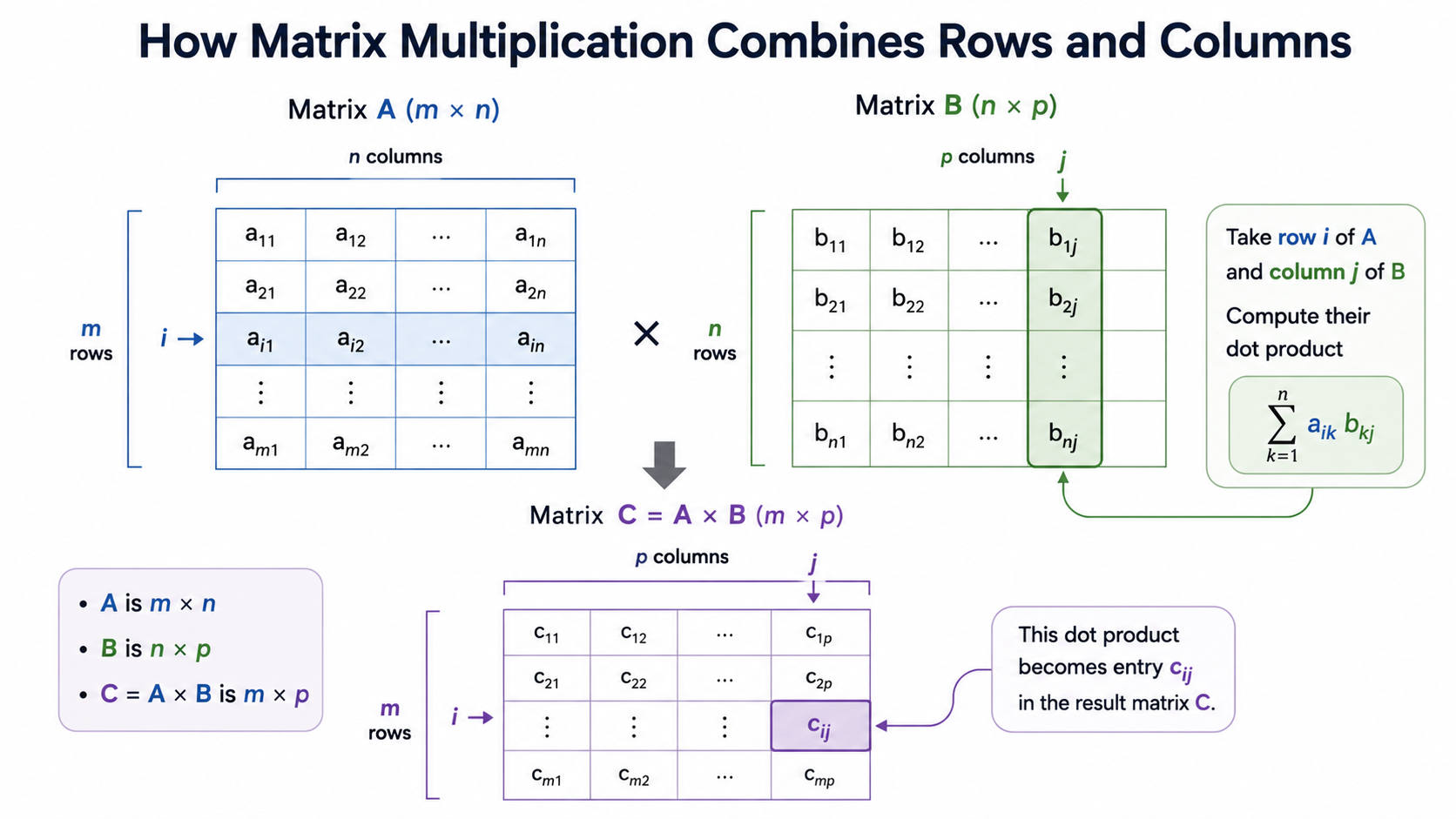
হাতে-কলমে উদাহরণ: ধরি এবং ।
যদি একটি লেয়ারের ওয়েট ম্যাট্রিক্স হয় এবং ইনপুট হয়, তবে ওই লেয়ারের প্রতিটি নিউরনের প্রি-অ্যাক্টিভেশন একটি মাত্র ধাপে ক্যালকুলেট করা যায়:
সহজ কথায়: -এর প্রতিটি সারি হলো এক একটি নিউরনের ওয়েট ভেক্টর। -কে দিয়ে গুণ করলে একসাথেই প্রতিটি সারির সাথে -এর ডট প্রোডাক্ট হয়ে যায় — আর সেটাই হলো সমস্ত নিউরনের ওয়েটেড সাম, যা একসাথেই বের হয়ে আসে। আর ঠিক এই কারণেই Deep Learning ফ্রেমওয়ার্কগুলো দ্রুত ম্যাট্রিক্স মাল্টিপ্লিকেশনের ওপর ভিত্তি করে তৈরি, এবং আধুনিক Deep Learning-এ কেন GPU (যারা ঠিক এই কাজেই ওস্তাদ) এত গুরুত্বপূর্ণ।
ম্যাট্রিক্স মাল্টিপ্লিকেশন কমিউটেটিভ (commutative) নয়
সাধারণত — এবং অনেক সময় শেপ-মিসম্যাচের কারণে এই দুটির যেকোনো একটি হয়তো আদৌ সংজ্ঞায়িতই হয় না। গুণ করার আগে সবসময় ডাইমেনশন চেক করুন; শূন্য থেকে Neural Network ইমপ্লিমেন্ট করার সময় এটি সবচেয়ে সাধারণ বাগগুলোর একটি।
ট্রান্সপোজ (The Transpose)
সহজ কথায়: ট্রান্সপোজ একটি ম্যাট্রিক্সকে তার কর্ণ বা ডায়াগোনাল (diagonal) বরাবর উল্টে দেয়, যার ফলে সারিগুলো কলামে এবং কলামগুলো সারিতে পরিণত হয়। যদি হয়, তবে হবে। Backpropagation-এ ট্রান্সপোজের খুব বেশি ব্যবহার দেখা যায়, কারণ গ্রেডিয়েন্টগুলো ফরোয়ার্ড পাসে ব্যবহৃত হওয়া একই ওয়েট ম্যাট্রিক্সের ভেতর দিয়েই পেছনের দিকে প্রবাহিত হয়, কিন্তু তখন তাদের ভূমিকা — এবং ডাইমেনশন — উল্টে যায়।
এলিমেন্ট-ভিত্তিক (হ্যাডামারড) প্রোডাক্ট (Element-wise / Hadamard Product)
যেখানে: এবং -এর শেপ অবশ্যই পুরোপুরি একই হতে হবে। ম্যাট্রিক্স মাল্টিপ্লিকেশনের মতো না হয়ে, এটি সরাসরি একই পজিশনে থাকা এন্ট্রিগুলোকে গুণ করে — কোনো ডট প্রোডাক্ট নেই, কোনো যোগ করাও নেই।
এটি কেন গুরুত্বপূর্ণ: Backpropagation-এর সময় যখন কোনো লেয়ারের আপস্ট্রিম গ্রেডিয়েন্টকে (upstream gradient) তার অ্যাক্টিভেশন ফাংশনের লোকাল ডেরিভেটিভের (local derivative) সাথে মেশানো হয়, তখন এই হ্যাডামারড প্রোডাক্ট কাজে আসে, কারণ অ্যাক্টিভেশন ফাংশনগুলো সবসময় এলিমেন্ট-ভিত্তিক বা একটি একটি করে নিউরনের ওপর প্রয়োগ করা হয়। backpropagation চ্যাপ্টারে আপনি ঠিক এই অপারেশনটিই দেখতে পাবেন, যা চিহ্ন দিয়ে লেখা থাকে।
এই দুটি গুণনকে গুলিয়ে ফেলবেন না
ম্যাট্রিক্স মাল্টিপ্লিকেশন () সারি আর কলামকে ডট প্রোডাক্টের মাধ্যমে মেলায় এবং ফলাফলের শেপটি পুরোপুরি পালটে দিতে পারে। অন্যদিকে হ্যাডামারড প্রোডাক্ট () করার জন্য শেপ একেবারে হুবহু এক হতে হয় এবং এটি শুধু এন্ট্রি ধরে ধরে গুণ করে, আর শেপটাও অপরিবর্তিত থাকে। এরা সম্পূর্ণ আলাদা সমস্যার সমাধান করে এবং একে অপরের বিকল্প হিসেবে ব্যবহার করা যায় না।
কিছু বিশেষ ম্যাট্রিক্স যা চিনে রাখা ভালো (Special Matrices Worth Recognizing)
| ম্যাট্রিক্স (Matrix) | বর্ণনা (Description) |
|---|---|
| আইডেন্টিটি (Identity / I) | কর্ণ বা ডায়াগোনালে শুধু 1 থাকে, বাকি সব জায়গায় 0 থাকে; এটি AI = IA = A শর্ত পূরণ করে |
| জিরো ম্যাট্রিক্স (Zero matrix) | প্রতিটি এন্ট্রিই শূন্য |
| ডায়াগোনাল ম্যাট্রিক্স (Diagonal matrix) | কর্ণ বাদে বাকি সব জায়গায় এন্ট্রি শূন্য |
| সিমেট্রিক ম্যাট্রিক্স (Symmetric matrix) | A = Aᵀ শর্তটি পূরণ করে |
| অর্থোগোনাল ম্যাট্রিক্স (Orthogonal matrix) | AᵀA = I শর্তটি পূরণ করে; এটি ভেক্টরের দৈর্ঘ্য এবং কোণ অপরিবর্তিত রাখে — এই কোর্সের পরের দিকে ওয়েট ইনিশিয়ালাইজেশন (weight initialization) বোঝার ক্ষেত্রে এর প্রাসঙ্গিকতা আছে |
আইগেনভ্যালু এবং আইগেনভেক্টর: একটি সংক্ষিপ্ত পরিচিতি (Eigenvalues and Eigenvectors: A Brief Introduction)
সাধারণত যখন একটি ম্যাট্রিক্স দিয়ে একটি ভেক্টর -কে গুণ করা হয়, তখন -এর দিক (direction) বদলে যায়। কিন্তু কিছু বিশেষ ভেক্টরের জন্য এমনটা ঘটে না — সেগুলো শুধু লম্বা বা ছোট হয়, দিক বদলায় না।
যেখানে: হলো একটি স্কয়ার বা বর্গাকার ম্যাট্রিক্স, হলো একটি আইগেনভেক্টর (eigenvector), এবং হলো তার সাথে সংশ্লিষ্ট আইগেনভ্যালু (eigenvalue) — একটি স্কেলার।
সহজ কথায়: দিয়ে -কে গুণ করলে সাধারণত যা হয় (দিক এবং দৈর্ঘ্য দুটোই বদলে যাওয়া) তার বদলে, একটি আইগেনভেক্টরের ক্ষেত্রে শুধু স্কেলিং ঘটে — ফলাফলটা মূল ভেক্টরেরই একটি -গুণ করা সংস্করণ। প্রতিটি স্কয়ার ম্যাট্রিক্সের নিজস্ব একটি বিশেষ দিকগুলোর সেট থাকে যেখানে এই সহজ আচরণটা ঘটে।
এটি কেন গুরুত্বপূর্ণ: ডিপ লার্নিং-এ আইগেনভ্যালু-আইগেনভেক্টরের সরাসরি ব্যবহার কম দেখা গেলেও, এর তাৎপর্য গভীর। হেসিয়ান ম্যাট্রিক্সের (Hessian matrix, যা ক্যালকুলাস চ্যাপ্টারে সংক্ষেপে উল্লেখ করা হয়েছে) আইগেনভ্যালুগুলো লস ল্যান্ডস্কেপের বক্রতা বা কার্ভেচার বর্ণনা করে — বড় পজিটিভ আইগেনভ্যালু মানে সেই দিকে ল্যান্ডস্কেপ খুব খাড়া (steep), আর ছোট আইগেনভ্যালু মানে প্রায় সমতল। এটাই ব্যাখ্যা করে কেন কিছু দিকে গ্রেডিয়েন্ট ডিসেন্ট দ্রুত এগোয় আর কিছু দিকে অত্যন্ত ধীরে। PCA (Principal Component Analysis)-এর মতো ডাইমেনশনালিটি রিডাকশন (dimensionality reduction) টেকনিকও পুরোপুরি ডেটার কোভ্যারিয়েন্স ম্যাট্রিক্সের আইগেনভেক্টরের ওপর ভিত্তি করে তৈরি।
এই মুহূর্তে হাতে-কলমে ক্যালকুলেট করা লাগবে না
আইগেনভ্যালু-আইগেনভেক্টর হাতে বের করার পদ্ধতি এই কোর্সের পরিধির বাইরে — এখানে শুধু ধারণাটা চেনা এবং কেন এটা গুরুত্বপূর্ণ তা বোঝাই যথেষ্ট। NumPy-এর np.linalg.eig() ফাংশন যেকোনো ম্যাট্রিক্সের জন্য এগুলো ক্যালকুলেট করে দিতে পারে।
Implementation
python
কয়েকটি জিনিস খেয়াল করার মতো: NumPy-তে @ অপারেটরটি ম্যাট্রিক্স মাল্টিপ্লিকেশন বোঝায়, যা * থেকে আলাদা (কারণ * হলো এলিমেন্ট-ভিত্তিক/হ্যাডামারড গুণনের জন্য)। X @ W.T + b ব্যাচ করা লাইনটি খেয়াল করুন: Python-এ দুটি উদাহরণের প্রতিটির জন্য লুপ চালানোর বদলে, একটি ম্যাট্রিক্স মাল্টিপ্লিকেশন একসাথেই দুটি উদাহরণের প্রি-অ্যাক্টিভেশন বের করে ফেলে, আর b স্বয়ংক্রিয়ভাবে প্রতিটি সারিতে ব্রডকাস্ট (broadcast) বা যোগ হয়ে যায়। ম্যানুয়াল লুপের বদলে ব্যাচ ধরে একসাথে ভেক্টরাইজড ফর্মে এই কাজ করার কারণেই Deep Learning ফ্রেমওয়ার্কগুলো দ্রুত গতির এবং GPU-অ্যাক্সিলারেটেড কম্পিউটেশনের সুবিধা নিতে পারে।
ব্যাচ করা শেপের কনভেনশন বা নিয়মটা মনে রাখবেন
একটি ব্যাচের প্রি-অ্যাক্টিভেশন সবসময় X @ W.T + b হিসেবে ক্যালকুলেট করুন, যেখানে X-এর শেপ হবে (batch_size, n_features) এবং W-এর শেপ হবে (n_outputs, n_features)। একেবারে গোড়া থেকে একটি লেয়ার ইমপ্লিমেন্ট করার সময় এই ট্রান্সপোজটা উল্টো করে ফেলা শেপ-মিসম্যাচের সবচেয়ে সাধারণ ভুলগুলোর একটি।
মূল বিষয়গুলো (Key Takeaways)
Key Takeaways
- ভেক্টর এবং ম্যাট্রিক্স হলো একটি MLP-এর বেসিক ডেটা স্ট্রাকচার: ইনপুট, ওয়েট, এবং বায়াস সবকিছুই এভাবে রিপ্রেজেন্ট করা হয়।
- ডট প্রোডাক্ট একটি নিউরনের ওয়েটেড সাম ক্যালকুলেট করে; আর ম্যাট্রিক্স মাল্টিপ্লিকেশন একটি পুরো লেয়ারের প্রি-অ্যাক্টিভেশনগুলো একসাথেই ক্যালকুলেট করে।
- নর্মস (Norms) (, ) ভেক্টরের আকার মাপে এবং এটি রেগুলারাইজেশন ও গ্রেডিয়েন্ট ক্লিপিংয়ের মূল ভিত্তি।
- ম্যাট্রিক্স মাল্টিপ্লিকেশনের জন্য ভেতরের ডাইমেনশনগুলো মিলে যাওয়া আবশ্যক এবং এটি কমিউটেটিভ বা বিনিময়যোগ্য নয় — খুব সাবধানে শেপ চেক করুন।
- হ্যাডামারড (এলিমেন্ট-ভিত্তিক) প্রোডাক্ট ম্যাট্রিক্স মাল্টিপ্লিকেশন থেকে সম্পূর্ণ আলাদা একটি অপারেশন, এবং Backpropagation ঠিক এটি ব্যবহার করেই গ্রেডিয়েন্টগুলোকে অ্যাক্টিভেশন ডেরিভেটিভের সাথে মেলায়।
- NumPy-এর
@অপারেটর এবং ব্রডকাস্টিং কোডের মধ্যে এই প্রতিটি অপারেশনকে দ্রুত ও সংক্ষিপ্ত করে তোলে।
সাধারণ ভুল ধারণা (Common Mistakes)
ম্যাট্রিক্স মাল্টিপ্লিকেশনকে হ্যাডামারড প্রোডাক্টের সাথে গুলিয়ে ফেলা
NumPy-তে W @ x এবং W * x সম্পূর্ণ আলাদা কাজ করে, আর এদের গুলিয়ে ফেললে কোনো ওয়ার্নিং ছাড়াই ভুল (তবে মাঝে মাঝে শেপ-কম্প্যাটিবল বা শেপ মিলে যাওয়ার মতো!) ফলাফল আসে। ম্যাট্রিক্স মাল্টিপ্লিকেশন সারি এবং কলামকে ডট প্রোডাক্টের মাধ্যমে মেলায়; আর হ্যাডামারড প্রোডাক্ট এন্ট্রি ধরে ধরে গুণ করে এবং এর জন্য হুবহু একই শেপ লাগে।
গুণ করার আগে ডাইমেনশন মিলেছে কি না তা চেক করতে ভুলে যাওয়া
কেবল তখনই সংজ্ঞায়িত করা যায় যখন -এর কলাম সংখ্যা -এর সারি সংখ্যার সমান হয় — এমনকী যদি কখনো এবং উভয়ই সংজ্ঞায়িত হয়, তবুও এরা প্রায় কখনোই সমান হয় না। সবসময় শেপ বা আকারগুলো চেক করে নিন, বিশেষ করে যখন সিঙ্গেল-এক্সাম্পল কোড থেকে ব্যাচ করা কোডে পরিবর্তন করছেন।
L1 এবং L2 নর্মকে একই জিনিস ভেবে গুলিয়ে ফেলা
L1 নর্ম (অ্যাবসোলিউট মানের যোগফল) এবং L2 নর্ম (স্কয়ারড মানের যোগফলের বর্গমূল) সাধারণত সম্পূর্ণ ভিন্ন সংখ্যা দেয় এবং তাদের আচরণও ভিন্ন। L1 রেগুলারাইজেশন স্পার্স (sparse) বা অনেক জিরো-সমৃদ্ধ ওয়েট তৈরি করার দিকে ঝোঁকে, যেখানে L2 রেগুলারাইজেশন সব ওয়েটকেই সমানভাবে ছোট রাখার দিকে ঝোঁকে। কোন নর্ম ব্যবহার করা হচ্ছে তার ওপর ভিত্তি করে মডেলের আচরণ সত্যিকার অর্থে বদলে যায়, তাই এই দুটোকে কখনোই বিনিময়যোগ্য (interchangeable) হিসেবে ধরে নেওয়া উচিত নয়।
ব্যাচ করা কোডে ট্রান্সপোজ ভুল জায়গায় দেওয়া
সিঙ্গেল-এক্সাম্পল ফর্মুলা থেকে ব্যাচ ফর্মুলায় যাওয়ার সময় ট্রান্সপোজ কোথায় বসবে তা ভুলে যাওয়া অত্যন্ত সাধারণ একটি ভুল। মনে রাখার সহজ উপায় হলো: X-এর শেপ সবসময় (batch_size, n_features), তাই W-কে অবশ্যই ট্রান্সপোজ করে তার শেপকে (n_features, n_outputs)-এ আনতে হবে যাতে ম্যাট্রিক্স মাল্টিপ্লিকেশনের ভেতরের ডাইমেনশন মিলে যায়।
ইন্টারভিউ কর্নার (Interview Corner)
Quick Check
বাস্তবে এটি কোথায় দেখা যায় (Where This Shows Up in Practice)
একটি MLP-এর প্রতিটি লেয়ারের ভেতর দিয়ে যাওয়ার প্রতিটি ফরোয়ার্ড পাস হলো একটি ম্যাট্রিক্স মাল্টিপ্লিকেশন এবং তার সাথে একটি বায়াস ভেক্টর যোগ করা; প্রতিটি ব্যাকওয়ার্ড পাস বা পেছনের দিকের প্রবাহে এই ট্রান্সপোজ করা ওয়েট ম্যাট্রিক্স এবং অ্যাক্টিভেশন ডেরিভেটিভের সাথে হ্যাডামারড প্রোডাক্ট বারবার ব্যবহার করা হয়। পরের চ্যাপ্টারে টুলকিটের বাকি অর্ধেকটা — অর্থাৎ ক্যালকুলাস (calculus) — তৈরি করা হবে, যাতে আমরা যখন backpropagation প্রমাণ করব, তখন "কী হচ্ছে" (এই চ্যাপ্টারের লিনিয়ার অ্যালজেব্রা) এবং "এটি কেন কাজ করছে" (পরের চ্যাপ্টারের ক্যালকুলাস), দুটোই আপনার কাছে খুব চেনা মনে হয়।