Chapter 16 of 25
Loss Functions
Teaching a network what 'wrong' means
18 min read
Created ২ আগ, ২০২৬
ভূমিকা (Motivation)
যেকোনো জিনিস পরিমাপ করতে না পারলে কোনো নেটওয়ার্ক সেই বিষয়ে নিজেকে উন্নত করতে পারে না। গ্রেডিয়েন্ট (gradient) ক্যালকুলেট করার আগে, কিংবা backpropagation-এর কাছে পেছনের দিকে প্রবাহিত করার মতো কিছু থাকার আগেই, এমন একটিমাত্র নম্বর বা সংখ্যার প্রয়োজন হয় যা বলে দেয় "তুমি ঠিক এতটাই ভুল ছিলে"। ওই নম্বরটিকেই বলা হয় লস (loss), এবং যে ফাংশনটি ওই নম্বরটি তৈরি করে — অর্থাৎ লস ফাংশন (loss function) — তা হলো পুরো ট্রেনিং পাইপলাইনের সবচেয়ে গুরুত্বপূর্ণ ডিজাইন সিদ্ধান্তগুলোর একটি। ভুল লস ফাংশন বেছে নিলে, এমনকি নিখুঁতভাবে ইমপ্লিমেন্ট করা কোনো নেটওয়ার্কও ভুল লক্ষ্যের দিকে ট্রেন হতে থাকবে।
এই চ্যাপ্টারটি বাস্তবে ব্যবহৃত লস ফাংশনগুলোর তালিকা তৈরি করে, এবং — যেহেতু Backpropagation চ্যাপ্টারে স্পষ্টভাবে কথা দেওয়া হয়েছিল — এটি খুব সাবধানে প্রতিপাদন করে বা ডিরাইভ (derive) করে দেখায় যে কেন সবচেয়ে সাধারণ দুটি জোড়া (বাইনারি ক্রস-এন্ট্রপির সাথে সিগময়েড, এবং ক্যাটাগরিক্যাল ক্রস-এন্ট্রপির সাথে সফটম্যাক্স) আউটপুট এরর সিগন্যালটিকে ভেঙে একেবারে একটি পরিষ্কার এবং সাধারণ রূপে, অর্থাৎ -এ নামিয়ে আনে।
একটি বাস্তব জীবনের উদাহরণ (A Real-Life Scenario)
ভাবুন তো, আপনি সম্পূর্ণ ভিন্ন ধরনের দুটি পরীক্ষার খাতা দেখছেন। একটি গাণিতিক বা নিউমেরিক পরীক্ষায় (যেমন তাপমাত্রা প্রেডিক্ট করা বা স্টকের দাম প্রেডিক্ট করা), "কতটা ভুল" এই ব্যাপারটা স্বাভাবিকভাবেই দূরত্বের পরিমাপের ওপর নির্ভর করে — ২ ডিগ্রি ভুল হওয়াটা ০.৫ ডিগ্রি ভুল হওয়ার চেয়ে বেশি খারাপ, আর এই ভুলের সাইজ বা আকারের সাথে সাথে শাস্তির পরিমাণটাও মসৃণভাবে ওঠা-নামা করা উচিত। এটা হলো রিগ্রেশন লস (regression losses)-এর জগৎ।
অন্যদিকে, একটি মাল্টিপল-চয়েস বা বহুনির্বাচনী পরীক্ষায় (যেমন এই ইমেইলটা কি স্প্যাম নাকি না, এটা কি বিড়াল, কুকুর নাকি পাখি), "কতটা ভুল" এই প্রশ্নটার ধরনই আলাদা — এখানে আপনি কোনো নির্দিষ্ট গাণিতিক দূরত্বে ভুল করছেন না, বরং আপনি সঠিক উত্তরটিতে আপনার কনফিডেন্স বা আত্মবিশ্বাস (confidence)-এর পরিমাণ ঠিক করেছেন, আর এখানে শাস্তির পরিমাণটা নির্ভর করা উচিত আপনি কতটা আত্মবিশ্বাসী ছিলেন এবং আপনার উত্তর ঠিক ছিল কি না, তার ওপর। এটা হলো ক্লাসিফিকেশন লস (classification losses)-এর জগৎ। লস ফাংশনগুলো খাতা দেখার এই দুটি দর্শনকেই গাণিতিকভাবে রূপ দেয়, আর এই চ্যাপ্টারটি দুই পাশের প্রধান প্রধান লসগুলো নিয়েই আলোচনা করে।
মূল ধারণা তৈরি করা (Building the Intuition)
- লস ফাংশন কোনো মনগড়া জিনিস নয় — এই চ্যাপ্টারের বেশিরভাগ লসই একটি Maximum Likelihood Estimation-এর যুক্তি থেকে প্রতিপাদন করা যায়: আসল লেবেলগুলো কীভাবে তৈরি হয় তার ওপর ভিত্তি করে একটি নির্দিষ্ট নয়েজ ডিস্ট্রিবিউশন (noise distribution) ধরে নিন, আর দেখবেন গণিতের ভেতর থেকে "পরিষ্কারভাবে সঠিক" লসটি এমনিতেই বেরিয়ে এসেছে।
- রিগ্রেশনের ক্ষেত্রে, এরর বা ভুলের (error) সাইজ এবং আকারটা বেশ গুরুত্বপূর্ণ: একে স্কয়ার (square) করলে বা বর্গ করলে বড় ভুলগুলোকে খুব কড়া শাস্তি দেওয়া হয়; অ্যাবসোলিউট ভ্যালু (absolute value) বা পরম মান নিলে সব ভুলকে সমানুপাতিকভাবে ধরা হয়; আর এই দুটোর সংমিশ্রণ বা হাইব্রিড (hybrid) করলে দুই জগতেরই সেরা সুবিধা পাওয়া যেতে পারে।
- ক্লাসিফিকেশনের ক্ষেত্রে, লস শুধু উত্তর সঠিক কি না তা-ই দেখে না, বরং উত্তরের কনফিডেন্স বা আত্মবিশ্বাসের (confidence) ওপরও গুরুত্ব দেয়: সঠিক উত্তরে ৫১% নিশ্চিত হওয়া আর ভুল উত্তরে ৫১% নিশ্চিত হওয়ার মধ্যে পুরষ্কারের পার্থক্য খুব সামান্য, কিন্তু ভুল উত্তরে ৯৯% নিশ্চিত হয়ে আত্মবিশ্বাসের সাথে ভুল করলে খুব কড়া শাস্তি দেওয়া হয়।
এর পেছনের গণিত: রিগ্রেশন লস (The Math Behind It: Regression Losses)
মিন স্কয়ারড এরর (Mean Squared Error / MSE)
MSE কোথা থেকে আসে: যদি আমরা ধরে নিই যে টার্গেটটি হিসেবে তৈরি হয়েছে, যেখানে গাউসিয়ান নয়েজ (Gaussian noise) হলো , তবে পর্যবেক্ষণ করা ডেটার লাইকলিহুড ম্যাক্সিমাইজ করলে — বা বলা যায় নেগেটিভ লগ-লাইকলিহুড মিনিমাইজ করলে — যেসব ধ্রুবক মিনিমাইজারকে প্রভাবিত করে না সেগুলোকে বাদ দেওয়ার পর, এটি হুবহু -এ পরিণত হয়। অন্য কথায়: MSE মিনিমাইজ করা আর গাউসিয়ান নয়েজ অনুমানের অধীনে Maximum Likelihood Estimation করা — দুটো আসলে হুবহু এক বিষয়।
সুবিধাসমূহ: মসৃণ বা স্মুথ (smooth), -এর সাপেক্ষে কনভেক্স (convex), স্কয়ার বা বর্গ করার কারণে বড় ভুলগুলোকে কড়া শাস্তি দেয়, এর গ্রেডিয়েন্ট খুব সিম্পল বা সহজ। অসুবিধাসমূহ: আউটলায়ার বা চরম ব্যতিক্রমী মানের (outliers) প্রতি খুবই সেনসিটিভ — একটি খুব বড় ভুল প্রেডিকশনকে স্কয়ার করলে তা পুরো লসকে একাই প্রভাবিত করে ফেলতে পারে। ব্যবহারের ক্ষেত্র: এটি হলো রিগ্রেশন লসের ডিফল্ট বা প্রথম পছন্দ, যখন এররগুলো মোটামুটি গাউসিয়ান হয় এবং আউটলায়ার বা চরম মানগুলো বড় কোনো চিন্তার বিষয় হয় না।
মিন অ্যাবসোলিউট এরর (Mean Absolute Error / MAE)
MAE গাউসিয়ানের বদলে ল্যাপ্লেস নয়েজ অনুমানের (Laplace noise assumption) অধীনে MLE-এর সাথে মিলে যায়। যেহেতু এখানে এরর বা ভুলগুলোকে স্কয়ার করা হয়বিধা হয় না, তাই বড় ভুলগুলো তুলনামূলকভাবে অতিরিক্ত বড় হয়ে যায় না — MAE আউটলায়ারদের ক্ষেত্রে বেশ রোবাস্ট (robust) বা শক্তপোক্ত। তবে এর ট্রেড-অফ হলো: ভুলের সাইজ যাই হোক না কেন, এর গ্রেডিয়েন্টের মান সবসময় নির্দিষ্ট বা কনস্ট্যান্ট থাকে, যা মিনিমামের কাছাকাছি গেলে সূক্ষ্ম কনভার্জেন্সকে ধীর এবং অস্থিতিশীল করে তুলতে পারে, আর ভুলের মান ঠিক শূন্য হলে এটি নন-ডিফারেনশিয়েবল (non-differentiable) হয়ে যায়।
হিউবার লস (Huber Loss)
হিউবার লস (Huber loss) দুই জগতেরই সেরা সুবিধাগুলোকে এক করে: ছোট ভুলের জন্য এটি MSE-এর মতো (মসৃণ, কোয়াড্রেটিক) আচরণ করে, আর বড় ভুলের জন্য MAE-এর মতো (রোবাস্ট, লিনিয়ার) আচরণ করে, ফলে এটি MSE-এর আউটলায়ার সেনসিটিভিটি এবং MAE-এর শূন্যতে থাকা চোখা ভাঁজ — দুটোকেই এড়ায়। রিইনফোর্সমেন্ট লার্নিংয়ের (reinforcement learning) ভ্যালু-ফাংশন (value-function) ট্রেনিংয়ে এটি খুব পরিচিত, এবং যে কোনো রিগ্রেশনের ক্ষেত্রে মসৃণতা ও রোবাস্টনেসের মধ্যে ভারসাম্য আনতে এটি ব্যবহৃত হয়।
এর পেছনের গণিত: ক্লাসিফিকেশন লস (The Math Behind It: Classification Losses)
বাইনারি ক্রস-এন্ট্রপি (Binary Cross-Entropy / BCE)
যেখান থেকে প্রতিপাদন করা হয়েছে: বার্নোলি (Bernoulli) ম্যাক্সিমাম লাইকলিহুডের যুক্তি থেকে — যদি প্রতিটি লেবেল ক্লাস 1-এ পড়ার প্রোবাবিলিটি নিয়ে করা একটি কয়েন টস হয়, তবে এটি হুবহু পর্যবেক্ষণ করা লেবেলগুলোর নেগেটিভ লগ-লাইকলিহুড। শর্ত: হতে হবে, যা সাধারণত একটি সিগময়েড আউটপুট অ্যাক্টিভেশন দিয়ে তৈরি করা হয়।
সিগময়েড + BCE সিম্প্লিফিকেশনের প্রতিপাদন (Deriving the Sigmoid + BCE Simplification)
Backpropagation চ্যাপ্টারে এই প্রতিপাদনটি দেখানোর কথা দেওয়া হয়েছিল: প্রমাণ করা যে সিগময়েড আউটপুটের সাথে BCE লস জোড়া বাঁধলে হয়।
একটি সিঙ্গেল উদাহরণের জন্য, যেখানে । প্রথমে, লসটিকে সরাসরি প্রেডিকশনের সাপেক্ষেই ডিফারেনশিয়েট করি:
এরপর সিগময়েডের ভেতর দিয়ে চেইন রুল প্রয়োগ করি, অ্যাক্টিভেশন ফাংশন চ্যাপ্টারে প্রমাণ করা ব্যবহার করে:
কেন এই কাটাকাটি হওয়াটা এত বড় ব্যাপার
লব (numerator) এবং হরের (denominator) অংশটুকু পুরোপুরি কাটাকাটি চলে যায়, ফলে একটি চমৎকার এবং সহজ রেজাল্ট পড়ে থাকে। ঠিক এ কারণেই সিগময়েড + BCE জোড়াটির ব্যবহার এত ব্যাপক: এটি একটি পরিষ্কার, নিউমেরিক্যালি স্ট্যাবল বা স্থিতিশীল গ্রেডিয়েন্ট তৈরি করে যেখানে শূন্যের কাছাকাছি কোনো সংখ্যা দিয়ে ভাগ করার ঝুঁকি থাকে না — যা নিশ্চিতভাবে হতো যদি আপনি খুব বেশি কনফিডেন্ট সঠিক বা ভুল প্রেডিকশনের ক্ষেত্রে এবং আলাদাভাবে ক্যালকুলেট করে সাধারণ গুণের মতো গুণ করতেন।
ব্যবহারের ক্ষেত্র: বাইনারি ক্লাসিফিকেশন, এটি সবসময় একটি সিগময়েড আউটপুট অ্যাক্টিভেশনের সাথেই জোড়া বাঁধা থাকে।
ক্যাটাগরিক্যাল ক্রস-এন্ট্রপি (Categorical Cross-Entropy / CCE)
যেখানে: হলো একটি ওয়ান-হট ভেক্টর (one-hot vector) (যেখানে আসল ক্লাসের ইনডেক্সে শুধু একটি 1 থাকে, বাকি সব 0), এবং হলো সফটম্যাক্স আউটপুট। যেখান থেকে প্রতিপাদন করা হয়েছে: ক্যাটাগরিক্যাল ডিস্ট্রিবিউশন MLE থেকে — যা ওপরের BCE প্রতিপাদনেরই সরাসরি মাল্টি-ক্লাস সাধারণ রূপ। যেহেতু হলো একটি ওয়ান-হট ভেক্টর, তাই ডাবল সাম (double sum) ভেঙে শুধু একটি টার্ম বা পদে চলে আসে: , যেখানে হলো আসল ক্লাস — লসটি মূলত মডেল কর্তৃক সঠিক ক্লাসের ওপর ধার্য করা প্রোবাবিলিটির নেগেটিভ লগ।
ওপরের BCE-এর মতোই হুবহু একই রকম প্রতিপাদন দিয়ে — সিগময়েড ডেরিভেটিভের জায়গায় সফটম্যাক্স জ্যাকোবিয়ান (softmax Jacobian) ব্যবহার করে — সফটম্যাক্স + CCE জোড়াটি হুবহু একই রকম পরিষ্কার সিম্প্লিফিকেশন বা সরলীকরণ তৈরি করে: । ঠিক এই কারণেই বাস্তবে সবসময় সফটম্যাক্স এবং ক্যাটাগরিক্যাল ক্রস-এন্ট্রপি একসাথে ব্যবহার করা হয়: সিগময়েড + BCE-কে যে দারুণ কাটাকাটিটি এতটা পরিষ্কার করে তুলেছিল, এখানে ঠিক সেই কাটাকাটিটিই ভেক্টর ফর্মে ফিরে আসে।
স্পার্স ক্যাটাগরিক্যাল ক্রস-এন্ট্রপি (Sparse categorical cross-entropy) কোনো আলাদা লস নয়
স্পার্স ক্যাটাগরিক্যাল ক্রস-এন্ট্রপি হুবহু একই গাণিতিক লস ক্যালকুলেট করে — পার্থক্য শুধু একটাই যে এখানে আসল লেবেলটিকে একটি ওয়ান-হট ভেক্টর (যেমন )-এর বদলে শুধু একটি ইন্টিজার (integer) বা পূর্ণসংখ্যা ক্লাসের ইনডেক্স হিসেবে (যেমন ) দেওয়া হয়। এটি পুরোপুরি একটি ইঞ্জিনিয়ারিং সুবিধা যা মেমরি বাঁচায় এবং একটি অতিরিক্ত ওয়ান-হট-এনকোডিং (one-hot-encoding) ধাপ এড়ায়; এর ফলে পাওয়া গ্রেডিয়েন্ট হুবহু একই হয়।
হিঞ্জ লস (Hinge Loss)
প্রেডিকশনটির সাইন বা চিহ্ন যদি সঠিক হয় এবং ডিসিশন বাউন্ডারি থেকে এর মার্জিন (margin) বা দূরত্ব যদি অন্তত 1 হয় (), তবে হিঞ্জ লস (Hinge loss) শূন্য হয়; আর প্রেডিকশনটি যদি ভুল বা আত্মবিশ্বাসের অভাবের অঞ্চলে প্রবেশ করে, তবে এটি লিনিয়ার বা রৈখিক হারে বাড়তে থাকে। এটি শুধু সঠিক ক্লাসিফিকেশন করতেই উৎসাহিত করে না, বরং বাউন্ডারির চারপাশে একটি আত্মবিশ্বাসী মার্জিন বা দূরত্ব বজায় রাখতেও সাহায্য করে। ঐতিহাসিকভাবে এটি সাপোর্ট ভেক্টর মেশিনের (Support Vector Machines) লস ফাংশন ছিল, এবং মার্জিন-ভিত্তিক বাইনারি ক্লাসিফিকেশনের জন্য মাঝেমধ্যে MLP-তেও এটি ব্যবহার করা হয়, যদিও বাস্তবে ক্রস-এন্ট্রপি এর চেয়ে বহুগুণ বেশি ব্যবহৃত হয়।
কুলব্যাক-লিবলার ডাইভারজেন্স এবং লেবেল স্মুথিং (Kullback-Leibler Divergence and Label Smoothing)
যেখানে: এটি দুটি প্রোবাবিলিটি ডিস্ট্রিবিউশন — আসল এবং প্রেডিক্ট করা — এর মধ্যকার "দূরত্ব" পরিমাপ করে (যদিও এটি প্রকৃত অর্থে গাণিতিক দূরত্ব নয়, কারণ এটি অ্যাসিমেট্রিক — )।
সহজ কথায়: যখন লেবেলগুলো ওয়ান-হট হয় (অর্থাৎ একটি স্ট্যান্ডার্ড ক্লাসিফিকেশন প্রবলেম), তখন এবং ক্যাটাগরিক্যাল ক্রস-এন্ট্রপি গ্র্যাডিয়েন্টের দিক থেকে সম্পূর্ণ সমতুল্য — এই দুটির পার্থক্য শুধু একটি ধ্রুবক টার্ম (যাকে বলা হয় -এর এনট্রপি), যা -এর সাপেক্ষে ডেরিভেটিভ নেওয়ার সময় শূন্য হয়ে যায়। ঠিক এই কারণে বাস্তবে CCE এবং KL divergence প্রায় বিনিময়যোগ্যভাবে ব্যবহার করা হয়।
KL divergence তখনই বেশি গুরুত্বপূর্ণ হয়ে ওঠে যখন টার্গেট নিজেই একটি ওয়ান-হট ভেক্টর নয়, বরং একটি "নরম" (soft) প্রোবাবিলিটি ডিস্ট্রিবিউশন — যেমন লেবেল স্মুথিং (label smoothing)-এ, যেখানে আসল ক্লাসের প্রোবাবিলিটি ইচ্ছাকৃতভাবে থেকে সামান্য কমিয়ে (যেমন ) বাকি ক্লাসগুলোর মধ্যে সমানভাবে ছড়িয়ে দেওয়া হয়। এটি মডেলকে অতিরিক্ত আত্মবিশ্বাসী (overconfident) হয়ে ওঠা থেকে বিরত রাখে এবং প্রায়ই জেনারেলাইজেশন (generalization) কিছুটা উন্নত করে।
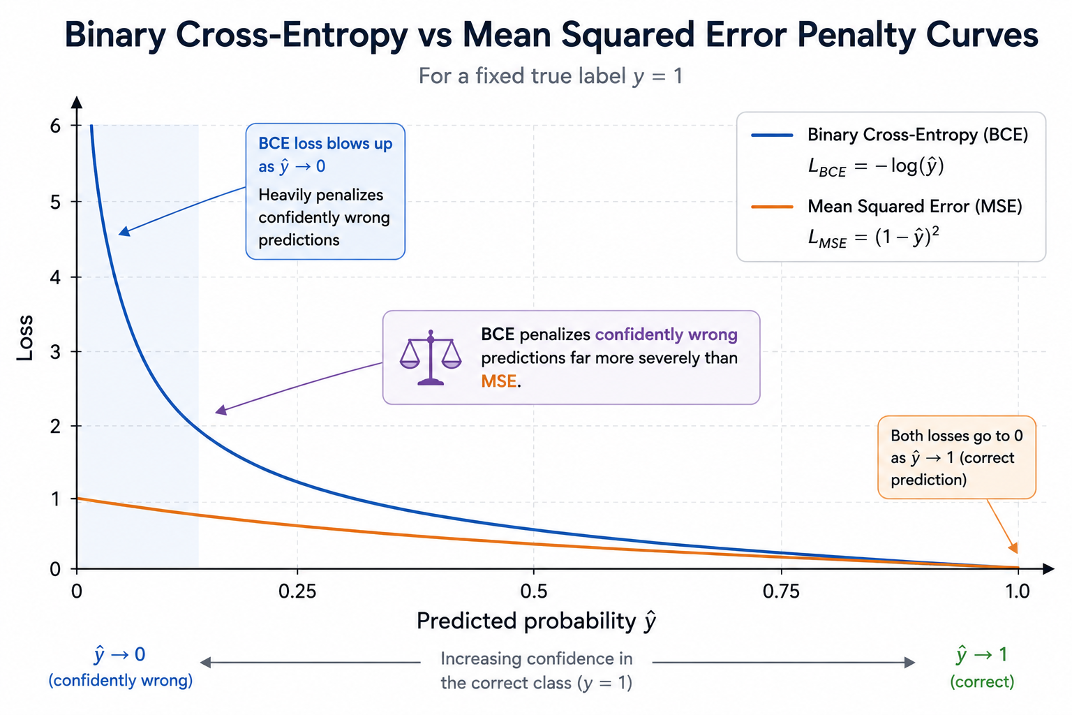
হাতে-কলমে গাণিতিক উদাহরণ: BCE বনাম MSE (Worked Numerical Example: BCE vs. MSE)
ধরা যাক এবং আসল লেবেলটি হলো :
এখন ধরা যাক মডেলটি খুব বাজেভাবে ভুল করেছে, আসল লেবেল -এর জন্য :
খেয়াল করে দেখুন, আত্মবিশ্বাসের সাথে করা ভুল প্রেডিকশনের (confidently-wrong prediction) জন্য BCE কতটা কড়া শাস্তি দিচ্ছে (0.223 থেকে 4.605 — প্রায় ২০ গুণ বৃদ্ধি), যেখানে MSE-এর শাস্তি তার চেয়ে অনেক কম (0.04 থেকে 0.980 — ২৫ গুণ বৃদ্ধি ঠিকই, কিন্তু এর অ্যাবসোলিউট বা পরম স্কেলটি অনেক ছোট এবং কম বৈষম্যমূলক)। ঠিক এই কারণেই ক্লাসিফিকেশনের জন্য সাধারণত ক্রস-এন্ট্রপিকে বেশি পছন্দ করা হয়: আত্মবিশ্বাসের সাথে করা ভুল প্রেডিকশনের ক্ষেত্রে এটি অনেক বেশি তীক্ষ্ণ গ্রেডিয়েন্ট তৈরি করে, যা দ্রুত ভুল শুধরাতে সাহায্য করে।
একটি সম্পূর্ণ মিনি-ব্যাচের ওপর গড় লস (Average Loss Over a Full Mini-Batch)
বাস্তবে লস কখনোই একটিমাত্র উদাহরণের ওপর গণনা করা হয় না — এটি সবসময় একটি মিনি-ব্যাচের ওপর গড় করা হয়। ধরা যাক আমাদের ৪টি উদাহরণের একটি বাইনারি ক্লাসিফিকেশন ব্যাচ আছে:
| উদাহরণ | আসল লেবেল y | প্রেডিকশন ŷ | একক BCE |
|---|---|---|---|
| 1 | 1 | 0.9 | 0.105 |
| 2 | 0 | 0.2 | 0.223 |
| 3 | 1 | 0.4 | 0.916 |
| 4 | 0 | 0.05 | 0.051 |
পুরো ব্যাচের লস হলো এই চারটি মানের গড়: । খেয়াল করুন উদাহরণ ৩ (আসল লেবেল , কিন্তু প্রেডিকশন মাত্র ) কীভাবে গড়টিকে সবচেয়ে বেশি টেনে ওপরে তুলেছে — এটাই ঠিক সেই আচরণ যা আমরা চাই: যে উদাহরণগুলোতে নেটওয়ার্ক সবচেয়ে বেশি ভুল করছে, ব্যাচ-গড় লস (এবং তাই গ্রেডিয়েন্ট) সেগুলোর প্রতি সবচেয়ে বেশি সংবেদনশীল হয়ে ওঠে।
Implementation
python
binary_cross_entropy এবং categorical_cross_entropy-এর ভেতরে থাকা eps ক্লিপিংটি শুধু সৌন্দর্যের জন্য দেওয়া হয়নি — নিচে ব্যাখ্যা করা ফেইলিওর মোড বা ব্যর্থতাকে এটি সরাসরি ঠেকিয়ে রাখে।
লগ নেওয়ার আগে সবসময় প্রোবাবিলিটিগুলোকে ক্লিপ করে নিন
যেহেতু ক্রস-এন্ট্রপিতে থাকে, তাই কোনো ক্লিপ না করা হুবহু 0.0 বা 1.0 মানের প্রেডিকশন — যা ফ্লোটিং-পয়েন্ট রাউন্ডিংয়ের (floating-point rounding) কারণে হতে পারে — বা NaN তৈরি করে, যা নীরবেই পুরো ট্রেনিং নষ্ট করে দেয়। কোডে কোনো ক্রস-এন্ট্রপি লস ক্যালকুলেট করার আগে সবসময় প্রেডিক্ট করা প্রোবাবিলিটিগুলোকে একেবারে শেষ প্রান্ত থেকে ক্লিপ করে নিন, যেমন রেঞ্জের ভেতরে।
তুলনামূলক ছক (Comparison Table)
| লস (Loss) | কাজ (Task) | নোট (Notes) |
|---|---|---|
| MSE | রিগ্রেশন (Regression) | আউটলায়ারের প্রতি সেনসিটিভ; গাউসিয়ান নয়েজের অধীনে MLE |
| MAE | রিগ্রেশন (Regression) | আউটলায়ারের ক্ষেত্রে রোবাস্ট; গ্রেডিয়েন্টের মান কনস্ট্যান্ট থাকে |
| হিউবার (Huber) | রিগ্রেশন (Regression) | MSE (0-এর কাছাকাছি) এবং MAE (0 থেকে দূরে)-এর আচরণের সংমিশ্রণ |
| বাইনারি ক্রস-এন্ট্রপি (Binary Cross-Entropy) | বাইনারি ক্লাসিফিকেশন | সিগময়েডের সাথে জোড়া বাঁধা থাকে; বার্নোলির অধীনে MLE |
| ক্যাটাগরিক্যাল ক্রস-এন্ট্রপি (Categorical Cross-Entropy) | মাল্টি-ক্লাস ক্লাসিফিকেশন | সফটম্যাক্সের সাথে জোড়া বাঁধা থাকে; ক্যাটাগরিক্যালের অধীনে MLE |
| স্পার্স ক্যাটাগরিক্যাল CE (Sparse Categorical CE) | মাল্টি-ক্লাস ক্লাসিফিকেশন | CCE-এর মতোই, তবে ওয়ান-হট ভেক্টরের বদলে ইন্টিজার লেবেল থাকে |
| হিঞ্জ (Hinge) | বাইনারি ক্লাসিফিকেশন (মার্জিন-ভিত্তিক) | ঐতিহাসিকভাবে SVM-এর সাথে ব্যবহৃত হয় |
মূল বিষয়গুলো (Key Takeaways)
Key Takeaways
- লস ফাংশনগুলো মনগড়া কিছু নয়: গাউসিয়ান নয়েজের অধীনে MLE থেকে MSE তৈরি হয়; বার্নোলি/ক্যাটাগরিক্যাল ডিস্ট্রিবিউশনের অধীনে MLE থেকে ক্রস-এন্ট্রপি লসগুলো তৈরি হয়।
- রিগ্রেশনে আউটলায়ারের ক্ষেত্রে রোবাস্টনেস বা শক্তপোক্ততা পেতে MAE এবং হিউবার লস কিছুটা মসৃণতা ছাড় দেয়।
- সিগময়েড + BCE এবং সফটম্যাক্স + CCE দুটোই খুব দারুণ গ্রেডিয়েন্ট সিম্প্লিফিকেশন তৈরি করে, যা ওপরে স্পষ্টভাবে প্রমাণ করা হয়েছে।
- স্পার্স ক্যাটাগরিক্যাল ক্রস-এন্ট্রপি গাণিতিকভাবে ক্যাটাগরিক্যাল ক্রস-এন্ট্রপির হুবহু সমান; এটি কেবল লেবেল এনকোডিং পরিবর্তন করে।
- হিঞ্জ লস মার্জিন-ভিত্তিক পৃথকীকরণকে উৎসাহিত করে, যা ঐতিহাসিকভাবে SVM-এর সাথে যুক্ত।
সাধারণ ভুল ধারণা (Common Mistakes)
ক্লাসিফিকেশনের জন্য MSE ব্যবহার করা
ক্রস-এন্ট্রপি যেভাবে আত্মবিশ্বাসের সাথে করা ভুল প্রেডিকশন আর হালকা ভুল প্রেডিকশনের মধ্যে পরিষ্কার পার্থক্য করতে পারে, MSE-এর গ্রেডিয়েন্ট তা পারে না, এবং এটি বার্নোলি বা ক্যাটাগরিক্যাল লেবেল ডিস্ট্রিবিউশনের অধীনে MLE-এর জন্য সঠিক লসও নয়। ক্লাসিফিকেশন কাজের জন্য ক্রস-এন্ট্রপি লস ব্যবহার করুন।
স্পার্স CCE এবং CCE যে একই লস, তা ভুলে যাওয়া
স্পার্স ক্যাটাগরিক্যাল ক্রস-এন্ট্রপিকে সম্পূর্ণ ভিন্ন এবং সস্তা কোনো অ্যাপ্রক্সিমেশন (approximation) ভেবে ভুল করাটা খুব সহজ। আসলে তা নয় — এটি হুবহু একই মান এবং গ্রেডিয়েন্ট ক্যালকুলেট করে; শুধু লেবেলের ফরম্যাট বা ধরনটি আলাদা হয়।
ব্যাচ সাইজ পরিবর্তন করার সময় লস স্কেল করতে ভুলে যাওয়া
যদি লস ফাংশনে সমষ্টি (sum) ব্যবহার করা হয় গড় (mean)-এর বদলে, তবে লস এবং গ্রেডিয়েন্ট উভয়েরই স্কেল সরাসরি ব্যাচ সাইজের সমানুপাতিক হয়ে যায় — অর্থাৎ ব্যাচ সাইজ পরিবর্তন করলে কার্যকরভাবে লার্নিং রেটও পরিবর্তিত হয়ে যায়। এই সূক্ষ্ম মিথস্ক্রিয়াটি ভুলে গেলে ব্যাচ সাইজ পরিবর্তনের পর ট্রেনিং হঠাৎ অস্থির হয়ে যেতে পারে। সবসময় স্পষ্টভাবে জেনে নিন আপনার ফ্রেমওয়ার্ক ডিফল্টভাবে sum নাকি mean ব্যবহার করছে।
ইন্টারভিউ কর্নার (Interview Corner)
Quick Check
বাস্তবে এটি কোথায় দেখা যায় (Where This Shows Up in Practice)
আপনার লেখা প্রতিটি ট্রেনিং লুপ (training loop) শুরুই হবে একটি লস ফাংশন বেছে নেওয়ার মাধ্যমে, আর সেই সিদ্ধান্তটি পুরো পাইপলাইন জুড়ে প্রভাব ফেলবে: এটি নির্ধারণ করবে যে কোন আউটপুট অ্যাক্টিভেশনটি সঠিক (BCE-এর সাথে সিগময়েড, CCE-এর সাথে সফটম্যাক্স, MSE/MAE/Huber-এর সাথে লিনিয়ার বা রৈখিক), এবং এটি নির্ধারণ করবে যে আউটপুট লেয়ারে backpropagation ঠিক কোন গ্রেডিয়েন্ট দিয়ে শুরু হবে। এই চ্যাপ্টারে প্রতিপাদন করা সেই পরিষ্কার সিম্প্লিফিকেশনটি শুধুই কোনো গাণিতিক কৌতূহল নয় — এটি প্রোডাকশনে থাকা প্রায় প্রতিটি ক্লাসিফিকেশন নেটওয়ার্কের ব্যাকওয়ার্ড পাসের (backward pass) আক্ষরিক অর্থেই প্রথম লাইনের কোড।