Chapter 2 of 25

Machine Learning Fundamentals

Teaching computers by example instead of by rule

17 min read

Motivation

Here's an experiment worth imagining: try to write a program, using only if/else statements, that reliably tells spam emails apart from real ones. Your first version might check for the word "lottery" or "free money." It'll work great — for about a week. Then spammers rephrase, misspell words on purpose, or hide text inside images, and your rulebook is obsolete. You patch it. They adapt again. You're now in an arms race you can't win by writing more rules, because the pattern you're chasing isn't really a fixed rule at all — it's a fuzzy, shifting statistical signature that would take thousands of hand-written exceptions to approximate, and even then it would never be complete.

Machine learning exists to get you out of that arms race entirely. Instead of writing the rules yourself, you show the computer thousands of labeled examples — this email is spam, this one isn't — and let an algorithm discover the pattern on its own. When spam evolves, you don't rewrite the program; you just feed it new examples.

A Real-Life Scenario

Picture a hospital that wants to predict which patients are at high risk of readmission within 30 days of discharge. There's no clean rule like "if age > 65 and diagnosis = X, readmit" that captures reality — readmission risk depends on dozens of interacting factors: medication history, lab results, social factors, prior admissions, and combinations of these that no human would think to write down as an explicit rule.

What the hospital does have is years of historical records: thousands of past patients, each with their intake data and a known outcome (readmitted or not). A machine learning model can comb through those records, discover which combinations of features actually predict readmission, and apply that discovered pattern to every new patient who walks through the door — no one had to author the rule, the data effectively wrote it.

Building the Intuition

The cleanest way to see what's new here is to compare it to how programming normally works.

1.Traditional programming

You supply Rules + Data, the computer produces Output. A human writes the logic by hand.

2.Machine learning

You supply Data + Output (the correct answers), and the computer produces the Rules. The algorithm discovers the logic itself.

That flip — handing the computer examples of the right answer instead of handing it the logic — is the entire idea. Everything else in machine learning is really just details about how to make that flip work reliably.

Tom Mitchell's formal definition

A computer program is said to learn from experience $E$ with respect to some task $T$ and performance measure $P$ , if its performance at $T$ , as measured by $P$ , improves with experience $E$ .

This definition looks abstract, but it's genuinely useful because it forces you to nail down three things before you build anything: what exactly is the task ( $T$ — is it spam detection? readmission prediction?), what data will the system learn from ( $E$ — a decade of hospital records? a year of labeled emails?), and how will you measure whether it's actually working ( $P$ — accuracy? something more nuanced?). Skipping any one of these three questions is a common way ML projects go wrong before they even start.

Types of Machine Learning

Not all learning problems look alike. They tend to fall into three broad families.

The three major categories of machine learning
Type	Description	Example
Supervised Learning	Learns a mapping from inputs to known, labeled outputs.	Predicting house prices (regression); classifying email as spam or not (classification).
Unsupervised Learning	Finds hidden structure in data that has no labels at all.	Grouping customers into segments by purchase behavior; reducing the dimensionality of data.
Reinforcement Learning	An agent learns to make sequential decisions by receiving rewards or penalties from an environment.	Training an agent to play a game or control a robot.

The Multi-Layer Perceptron you'll build throughout this course is a general-purpose function approximator, and it shows up most often inside the supervised learning framework — for both regression and classification. But don't file it away as "only for supervised learning": MLP-shaped components also appear inside unsupervised architectures (like autoencoders) and reinforcement learning systems (approximating value functions or policies). The math you're about to learn is more portable than any one category suggests.

Supervised learning, a little more precisely

In supervised learning, you're handed a training dataset of $N$ input-output pairs:

\mathcal{D} = \{ (\mathbf{x}^{(1)}, y^{(1)}), (\mathbf{x}^{(2)}, y^{(2)}), \dots, (\mathbf{x}^{(N)}, y^{(N)}) \}

where $\mathbf{x}^{(i)}$ is the feature vector for example $i$ , and $y^{(i)}$ is its known label. The goal is to learn a function $f_\theta$ — for an MLP, $\theta$ is shorthand for all its weights and biases, which you'll meet properly in the next few chapters — such that $f_\theta(\mathbf{x}^{(i)}) \approx y^{(i)}$ for every training example, and, critically, such that $f_\theta$ still works well on brand-new inputs it never saw during training. Getting the first part right is easy. Getting the second part right is most of what this course is really about.

If $y$ is a continuous number (house price, temperature), the task is called regression.
If $y$ is a discrete category (spam / not spam), the task is called classification.

Core Concepts You'll Need Constantly

Features and labels

A feature is a measurable input property (square footage of a house, exclamation marks in an email). A label is the thing you're trying to predict (sale price, spam or not). Historically, deciding which features to feed a model — called feature engineering — was one of the most labor-intensive parts of machine learning, requiring deep domain expertise. One of deep learning's biggest advantages, which the next chapter explores properly, is that it can learn useful features directly from raw data, cutting out much of that manual work.

Training, validation, and test sets

The Three-Way Data Split

A dataset is typically divided into three disjoint subsets: the training set (used to fit the model's parameters), the validation set (used to tune hyperparameters and monitor generalization during development), and the test set (used exactly once, at the very end, to get an honest, unbiased estimate of performance on new data). Intuition: Think of the training set as the textbook you study from, the validation set as practice exams you use to figure out what to study more, and the test set as the real final exam — one you only take once, and never get to see in advance.

Never tune using the test set

A very common beginner mistake is tweaking hyperparameters based on test-set performance. That silently leaks information from the test set into your model-selection process, and the "final" accuracy you report ends up overly optimistic — it no longer measures generalization to genuinely unseen data. Reserve the test set until the very last step, and touch it exactly once.

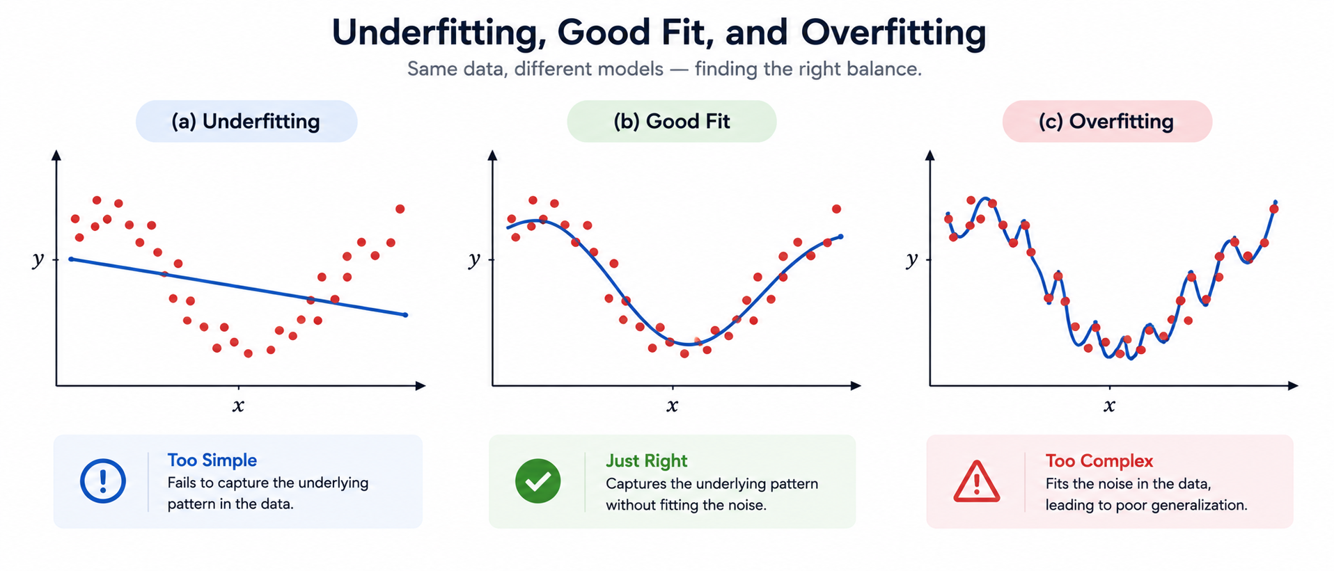
Underfitting and overfitting

These two failure modes will follow you through the entire course, so it's worth getting a rock-solid intuition for them now.

Definitions

Underfitting happens when a model is too simple to capture the real pattern in the data — it performs poorly on both the training set and new data. Overfitting happens when a model is too complex relative to the amount of training data — it starts memorizing noise and quirks specific to the training set, producing excellent training performance but poor performance on anything new.

Underfitting, Good Fit, and OverfittingIllustration coming soon

Underfitting misses the underlying trend entirely; a good fit captures the trend while ignoring noise; overfitting memorizes every point, including the noise.

The bias-variance tradeoff

Bias-Variance Decomposition

\mathbb{E}\left[(y - f_\theta(\mathbf{x}))^2\right] = \big(\text{Bias}[f_\theta(\mathbf{x})]\big)^2 + \text{Var}[f_\theta(\mathbf{x})] + \sigma^2

The General Machine Learning Workflow

1.Data Collection

Gather raw examples relevant to the task.

2.Data Preprocessing

Clean, normalize, and transform raw data into a usable form.

3.Train / Val / Test Split

Partition the data so training, tuning, and final evaluation never contaminate each other.

4.Model Training

Fit the model's parameters on the training set.

5.Evaluation

Measure performance on the validation set.

6.Hyperparameter Tuning

Adjust settings based on validation performance, then retrain.

7.Deployment / Monitoring

Ship the model and keep watching its real-world performance over time.

This exact pipeline applies directly to training a Multi-Layer Perceptron — every stage here reappears, in more mathematical detail, once you start actually building one.

Key Takeaways

Machine learning flips traditional programming: instead of Rules + Data → Output, it's Data + Output → Rules, discovered automatically.
Tom Mitchell's definition forces precision about three things: the task $T$ , the experience $E$ , and the performance measure $P$ .
The three major types are supervised, unsupervised, and reinforcement learning; the MLP is used primarily — but not exclusively — in supervised learning.
Data is split into training, validation, and test sets specifically so you can get an honest estimate of how well a model generalizes.
Overfitting (high variance) and underfitting (high bias) are the two failure modes every model — including every MLP you'll ever train — must be guarded against.

Common Mistakes

Confusing feature engineering with the model itself

Spending all your effort on the model while feeding it poorly chosen features (or vice versa) is a classic beginner trap. Both matter — though as you'll see next chapter, deep learning shifts a lot of this burden onto the model itself.

Judging a model only by training accuracy

A model with 99% training accuracy and 60% test accuracy hasn't learned the task — it's memorized the training set. Always report performance on data the model never trained on.

Interview Corner

Quick Check

1. According to Tom Mitchell's definition, what three things must be precisely specified for a learning problem?

2. A model achieves 99% accuracy on its training set but only 61% on new, unseen data. What is this a textbook symptom of?

Where This Shows Up in Practice

Every supervised model you'll ever deploy — from a simple linear regressor to the deepest neural network — lives or dies by the concepts in this chapter: a properly measured task, a clean data split, and a healthy position on the bias-variance spectrum. The Multi-Layer Perceptron doesn't get a pass on any of this; if anything, its flexibility makes overfitting a bigger risk, which is exactly why later chapters on regularization exist. Get comfortable with these fundamentals now — you'll lean on them in every chapter that follows.