Chapter 13 of 25

MLP Architecture

Layers, neurons, and how information flows forward

19 min read

Motivation

A single perceptron can only ever draw one straight line through the data. That's fine for problems where one line is enough — but the moment a problem needs a curved boundary, or several boundaries stitched together (like recognizing a handwritten digit, or telling apart a cat from a dog in a photo), one perceptron simply doesn't have the expressive power. You already know why: it's a single linear cut, nothing more.

The fix seems obvious at first glance — just stack perceptrons on top of each other, layer after layer. But how exactly do you wire them together, what flows between them, and does stacking even help at all if you do it carelessly? This chapter answers all three questions precisely: it gives the Multi-Layer Perceptron its full, formal architecture, and derives the forward propagation equations that turn a raw input into a prediction.

A Real-Life Scenario

Think about how a hospital triage system might assess a patient. A single simple rule like "high temperature → flag as sick" is a one-line perceptron-style decision, and it misses a lot: a patient with a mildly high temperature but dangerously low blood pressure and an elevated heart rate should also be flagged, even though no single measurement alone crosses an obvious threshold.

A more realistic assessment happens in stages. First, a nurse combines several vitals into intermediate judgments — "is the cardiovascular picture concerning?", "is there a possible infection?" Then a doctor combines those intermediate judgments into a final decision. That's exactly the shape of a Multi-Layer Perceptron: raw inputs get combined into intermediate representations by a hidden layer, and those intermediate representations get combined again by the next layer, all the way to a final prediction.

Building the Intuition

An MLP is organized into layers: an input layer that just holds the raw data (no computation happens here), one or more hidden layers that build up increasingly useful intermediate representations, and an output layer that produces the final prediction.
Every hidden and output layer neuron does the same two-step job you already know from the perceptron: take a weighted sum of everything coming in from the previous layer (plus a bias), then apply an activation function.
The key difference from a single perceptron isn't the individual neuron — it's that the output of one layer becomes the input to the next. Information strictly flows forward, layer by layer, which is exactly why this is called a "feedforward" network.
Crucially, every layer needs a nonlinear activation function. If every layer only did a linear weighted sum, then no matter how many layers you stack, the whole network could always be collapsed back down into a single linear layer — depth would buy you nothing at all. We prove this below.

Multi-Layer Perceptron Architecture and NotationIllustration coming soon

Notation used throughout: x is the input, a_j^[ℓ] denotes the activation of neuron j in layer ℓ, and ŷ is the network's final output.

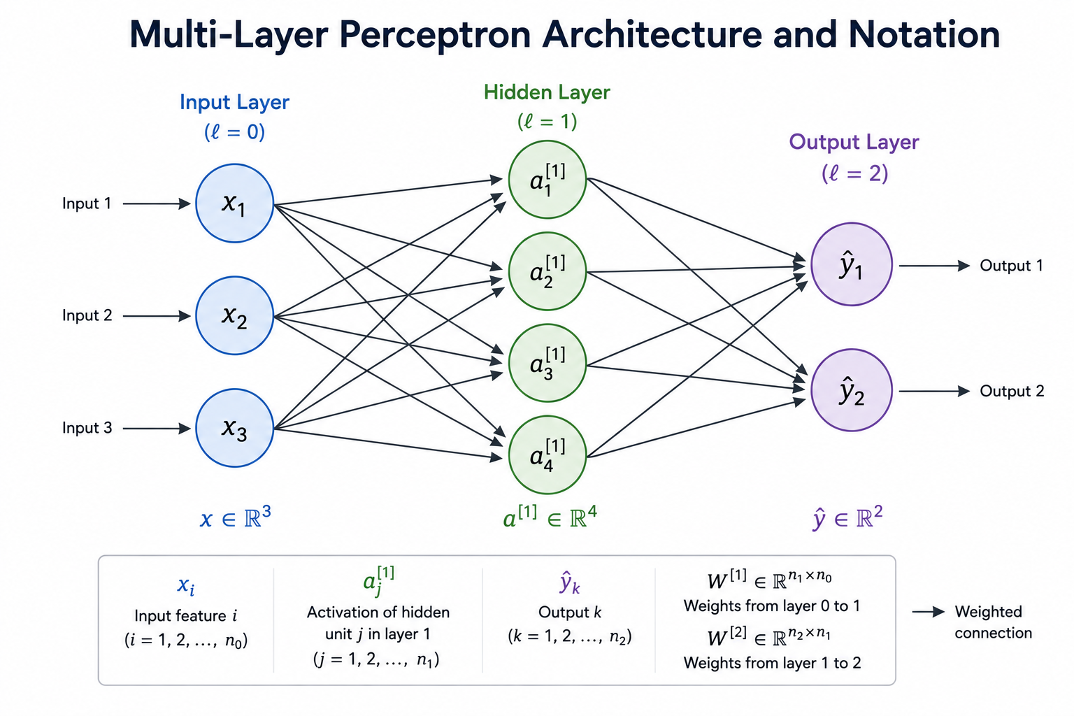
The Math Behind It

Layer Components

Component	Role
Input layer	Holds the raw feature vector $\mathbf{x}\in\mathbb{R}^{n_0}$ ; performs no computation and has no weights of its own
Hidden layer(s)	Transform the input into increasingly abstract representations via $\mathbf{z}^{[\ell]}=\mathbf{W}^{[\ell]}\mathbf{a}^{[\ell-1]}+\mathbf{b}^{[\ell]}$ followed by a nonlinear activation
Output layer	Produces the final prediction $\hat{\mathbf{y}}$ ; its activation depends on the task (sigmoid for binary classification, softmax for multi-class, linear/identity for regression)
Weights $\mathbf{W}^{[\ell]}$	Learnable parameters controlling the strength of each connection between layer $\ell-1$ and layer $\ell$
Biases $\mathbf{b}^{[\ell]}$	Learnable per-neuron offsets, letting a neuron shift its activation threshold independently of its inputs
Activation $\varphi^{[\ell]}$	Nonlinear function applied element-wise to $\mathbf{z}^{[\ell]}$

Don't underestimate the bias

Without a bias term, every layer's decision boundary is forced to pass through the origin — a severe, unnecessary restriction on what the network can represent. Always include and train bias terms unless there's a specific architectural reason not to.

Why Nonlinearity Is Not Optional

Necessity of Nonlinearity

\mathbf{a}^{[1]} = \mathbf{W}^{[1]}\mathbf{x}+\mathbf{b}^{[1]}

This is why depth matters at all

Without nonlinear activations, no amount of depth adds any representational power beyond a single-layer perceptron — and a single linear layer can't even solve XOR. Nonlinear activation functions are precisely what allow depth to matter. The next chapter studies the specific choices (sigmoid, tanh, ReLU, and friends) in full detail.

Forward Propagation

Forward Propagation, Layer by Layer

\mathbf{z}^{[\ell]} = \mathbf{W}^{[\ell]}\mathbf{a}^{[\ell-1]} + \mathbf{b}^{[\ell]}, \qquad \mathbf{a}^{[\ell]} = \varphi^{[\ell]}\big(\mathbf{z}^{[\ell]}\big), \qquad \ell = 1, \dots, L

Get the shapes right before writing any code

A layer with $n_{\ell-1}$ inputs and $n_\ell$ outputs must have $\mathbf{W}^{[\ell]}$ of shape $(n_\ell, n_{\ell-1})$ and $\mathbf{b}^{[\ell]}$ of shape $(n_\ell,)$ . Writing out every weight matrix's shape before implementing a network eliminates the majority of shape-mismatch bugs.

Interactive: See a Decision Boundary Move

Before tackling a full multi-layer example, it helps to see how a single neuron's weights and bias shape its decision boundary — the same building block that gets stacked, layer after layer, into a full MLP.

Weight Adjustment Playground

Adjust w1, w2, and the bias of a single neuron and watch its decision boundary move live over a fixed set of sample points.

w11.0w21.0b0.0

z = 1.0·x + 1.0·y + 0.0

Points shift between the two colors the moment the boundary line crosses them — this is the entire "decision" a single neuron makes.

Worked Numerical Example: Forward Propagation Through a 2-Layer Network

This exact worked example is referenced throughout the rest of this course, including in the Backpropagation chapter — so it's worth tracing carefully by hand. Consider a network with 2 inputs, one hidden layer of 2 neurons (sigmoid activation), and one output neuron (sigmoid activation, for binary classification).

Given:

\mathbf{x} = \begin{bmatrix}1.0 \\ 0.5\end{bmatrix}, \quad \mathbf{W}^{[1]} = \begin{bmatrix}0.3 & -0.2 \\ 0.5 & 0.1\end{bmatrix}, \quad \mathbf{b}^{[1]} = \begin{bmatrix}0.1 \\ -0.1\end{bmatrix}, \quad \mathbf{W}^{[2]} = \begin{bmatrix}0.8 & -0.6\end{bmatrix}, \quad b^{[2]} = 0.2

Layer 1 pre-activation:

\mathbf{z}^{[1]} = \mathbf{W}^{[1]}\mathbf{x}+\mathbf{b}^{[1]} = \begin{bmatrix}(0.3)(1.0)+(-0.2)(0.5) \\ (0.5)(1.0)+(0.1)(0.5)\end{bmatrix} + \begin{bmatrix}0.1\\-0.1\end{bmatrix} = \begin{bmatrix}0.30\\0.45\end{bmatrix}

Layer 1 activation (sigmoid, $\sigma(x)=\frac{1}{1+e^{-x}}$ ):

\mathbf{a}^{[1]} = \begin{bmatrix}\sigma(0.30)\\\sigma(0.45)\end{bmatrix} \approx \begin{bmatrix}0.5744\\0.6106\end{bmatrix}

Layer 2 pre-activation:

z^{[2]} = \mathbf{W}^{[2]}\mathbf{a}^{[1]}+b^{[2]} = (0.8)(0.5744)+(-0.6)(0.6106)+0.2 \approx 0.4595 - 0.3664 + 0.2 = 0.2931

Layer 2 activation (final prediction):

\hat{y} = \sigma(0.2931) \approx 0.5728

The network predicts a probability of about $0.573$ that the input belongs to the positive class. Hold onto these exact numbers — $\mathbf{z}^{[1]}=(0.30,0.45)$ , $\mathbf{a}^{[1]}=(0.5744,0.6106)$ , $z^{[2]}=0.2931$ , $\hat{y}=0.5728$ — the Backpropagation chapter picks up precisely where this leaves off, using this same forward pass to compute gradients.

Implementing It

import numpy as np
 
def sigmoid(z):
    return 1 / (1 + np.exp(-z))
 
x  = np.array([1.0, 0.5])
W1 = np.array([[0.3, -0.2], [0.5, 0.1]])
b1 = np.array([0.1, -0.1])
W2 = np.array([[0.8, -0.6]])
b2 = np.array([0.2])
 
z1 = W1 @ x + b1
a1 = sigmoid(z1)
 
z2 = W2 @ a1 + b2
a2 = sigmoid(z2)          # final prediction
 
print("z1 =", z1)
print("a1 =", a1)
print("z2 =", z2)
print("y_hat =", a2)

Running this reproduces the hand calculation exactly: z1 = [0.3, 0.45], a1 ≈ [0.5744, 0.6106], z2 ≈ 0.2931, y_hat ≈ 0.5728. Notice how each layer is just two lines — one matrix-vector multiply plus a bias, then an activation — repeated once per layer.

Standard Notation Reference

Symbol	Meaning
$L$	Number of layers with weights (excluding the input layer)
$n_\ell$	Number of neurons in layer $\ell$
$\mathbf{W}^{[\ell]}\in\mathbb{R}^{n_\ell\times n_{\ell-1}}$	Weight matrix of layer $\ell$
$\mathbf{b}^{[\ell]}\in\mathbb{R}^{n_\ell}$	Bias vector of layer $\ell$
$\mathbf{z}^{[\ell]}$	Pre-activation of layer $\ell$
$\mathbf{a}^{[\ell]}$	Activation (post-nonlinearity output) of layer $\ell$
$\hat{\mathbf{y}} = \mathbf{a}^{[L]}$	Network's final prediction

Key Takeaways

An MLP consists of an input layer, one or more hidden layers, and an output layer, each hidden/output layer defined by weights, a bias, and an activation function.
Without nonlinear activations, any depth of stacked linear layers collapses to a single linear transformation — proven explicitly above.
Forward propagation computes $\mathbf{z}^{[\ell]}=\mathbf{W}^{[\ell]}\mathbf{a}^{[\ell-1]}+\mathbf{b}^{[\ell]}$ then $\mathbf{a}^{[\ell]}=\varphi^{[\ell]}(\mathbf{z}^{[\ell]})$ , layer by layer, from input to output.
Correct matrix shapes — $\mathbf{W}^{[\ell]}$ as $(n_\ell, n_{\ell-1})$ and $\mathbf{b}^{[\ell]}$ as $(n_\ell,)$ — should always be verified before implementation.

Common Mistakes

Forgetting the input layer does no computation

Layer 0 simply holds $\mathbf{x}$ . It's easy to accidentally count it as a "real" layer with weights when sizing a network — it isn't one.

Mixing up W^[ℓ]'s row and column dimensions

$\mathbf{W}^{[\ell]}$ has shape $(n_\ell, n_{\ell-1})$ — outputs by inputs, not the other way around. Transposing this by accident is one of the most common shape-mismatch bugs when implementing a network from scratch.

Interview Corner

Quick Check

1. Why must an MLP use nonlinear activation functions in its hidden layers?

2. In the worked forward-propagation example, what is a^[1] after applying the sigmoid activation?

Where This Shows Up in Practice

Every image classifier, language model, and recommendation system ultimately rests on this exact forward propagation recipe, just with far more layers and far more exotic layer types layered on top. Understanding this simple two-layer example by hand is the foundation for everything that follows: backpropagation computes gradients by running this same computation graph backward, and every architectural choice in later chapters — activation functions, loss functions, optimizers — plugs directly into the $\mathbf{z}^{[\ell]}, \mathbf{a}^{[\ell]}$ machinery defined here.