Chapter 12 of 25
Optimization Theory
How a network actually searches for good weights
18 min read
Created ২ আগ, ২০২৬
ভূমিকা (Motivation)
ধরুন, আপনি রাতের বেলা কুয়াশায় ঢাকা কোনো এক পাহাড়ি রেঞ্জের ওপর দাঁড়িয়ে আছেন, আর আপনার একমাত্র লক্ষ্য হলো সবচেয়ে নিচু উপত্যকায় পৌঁছানো। কিন্তু আপনি চারপাশে কয়েক ফুটের বেশি কিছুই দেখতে পাচ্ছেন না। আপনি কেবল নিজের পায়ের নিচের ঢাল বা স্লোপটুকু অনুভব করতে পারেন, নিচের দিকে এক পা ফেলতে পারেন, আবার ঢাল অনুভব করতে পারেন, এবং এই কাজটির পুনরাবৃত্তি করতে পারেন। ব্যস, এটুকুই। এটাই হলো আপনার পুরো স্ট্র্যাটেজি।
এই অন্ধের মতো, ধাপে ধাপে নিচে নামার বিষয়টা শুধু যে একটা আলগা মেটাফোর বা রূপক, তা নয় — প্রতিবার যখন একটি নিউরাল নেটওয়ার্ক ট্রেন বা প্রশিক্ষিত হয়, তখন প্রায় হুবহু এটাই ঘটে। "একটি মডেলকে ট্রেন করা" কথাটি শুনতে খুব রহস্যময় বা প্রায় জাদুকরী কোনো প্রক্রিয়া বলে মনে হলেও, এর বাইরের কঠিন শব্দগুলোর আড়ালে এটি খুব স্পষ্ট একটি কাজ: সেই নম্বরগুলোর (ওয়েটস এবং বায়াস বা weights and biases) সেট খুঁজে বের করা যা একটি লস ফাংশনকে (loss function) যতটা সম্ভব ছোট করে তোলে। আপনি এ পর্যন্ত যত নিউরন, যত লেয়ার, যত অ্যাক্টিভেশন ফাংশন সম্পর্কে পড়েছেন, সেগুলোর আসল উদ্দেশ্যই হলো শেষ পর্যন্ত কোনো এক প্রক্রিয়ার মাধ্যমে সবকিছুর জন্য ভালো মান বা ভ্যালু খুঁজে বের করা। এই চ্যাপ্টারটি হলো সেই "কোনো এক প্রক্রিয়াটি" নিয়েই।
একটি বাস্তব জীবনের উদাহরণ (A Real-Life Scenario)
ভাবুন তো, একটি ডেলিভারি কোম্পানি প্রতিদিন তাদের ট্রাকগুলোর মোট চলার দূরত্ব কমানোর চেষ্টা করছে। এমন কোনো ফর্মুলা নেই যা একবার সমাধান করলেই কাজ শেষ — এখানকার "খরচ" বা "cost" (অর্থাৎ মোট দূরত্ব) শত শত পরস্পর নির্ভরশীল সিদ্ধান্তের ওপর নির্ভর করে (কোন ট্রাক কোথায় যাবে, কোন ক্রমে বা অর্ডারে যাবে), আর সম্ভাব্য খরচের ল্যান্ডস্কেপটি বা ভূদৃশ্যটি বেশ এবড়োখেবড়ো, যা ভালো-খারাপ বিভিন্ন অঞ্চলে ভরা, এবং সবচেয়ে ভালোটিতে পৌঁছানোর কোনো সহজ বা শর্টকাট পথ নেই। কোম্পানির প্ল্যানাররা রুটগুলোকে একটু একটু করে পরিবর্তন করেন বা নাড়াচাড়া করেন, তারপর দেখেন যে মোট দূরত্ব কমল কি না, আবার একটু পরিবর্তন করেন, এবং এই কাজটির পুনরাবৃত্তি করতে থাকেন।
একটি নিউরাল নেটওয়ার্কের ট্রেনিং লুপ বা training loop ঠিক একই গল্প, শুধু পার্থক্য হলো এখানকার "রুট" বা পথগুলো হলো মিলিয়ন মিলিয়ন ওয়েটস, আর "মোট দূরত্ব" হলো লস ফাংশন। একজন মানুষ নিজে হাতে নাড়াচাড়া করার বদলে, এখানে গ্রেডিয়েন্ট ডিসেন্ট (gradient descent) স্বয়ংক্রিয়ভাবে সেই নাড়াচাড়ার কাজটা করে, যেখানে অনুমানের বদলে ক্যালকুলাসের বা calculus-এর সাহায্য নেওয়া হয়।
মূল ধারণা তৈরি করা (Building the Intuition)
কোনো ইকুয়েশন বা সমীকরণ ধরার আগেই, এই তিনটি ধারণা মনে গেঁথে নিন:
- ট্রেনিং হলো একটি অনুসন্ধান বা search, কোনো সাধারণ হিসাব-নিকাশ বা calculation নয়। এমন কোনো ম্যাজিক ফর্মুলা নেই যা আপনাকে সরাসরি সেরা ওয়েটসগুলো বের করে দেবে — নেটওয়ার্ককে ধাপে ধাপে চেষ্টা করতে হয়, মাপতে হয় এবং নিজেকে মানিয়ে নিতে হয়।
- লস ফাংশন (loss function)-টিই হলো সেই ল্যান্ডস্কেপ বা ভূদৃশ্য। ওয়েটসের সম্ভাব্য প্রতিটি সেটিং হলো এই ল্যান্ডস্কেপের ওপর একটি নির্দিষ্ট পয়েন্ট বা বিন্দু, আর ওই পয়েন্টের উচ্চতাটি নির্দেশ করে যে নেটওয়ার্কের প্রেডিকশনগুলো কতটা খারাপ। ট্রেনিং করার অর্থ হলো এই ল্যান্ডস্কেপ ধরে নিচের দিকে হাঁটা বা নামা।
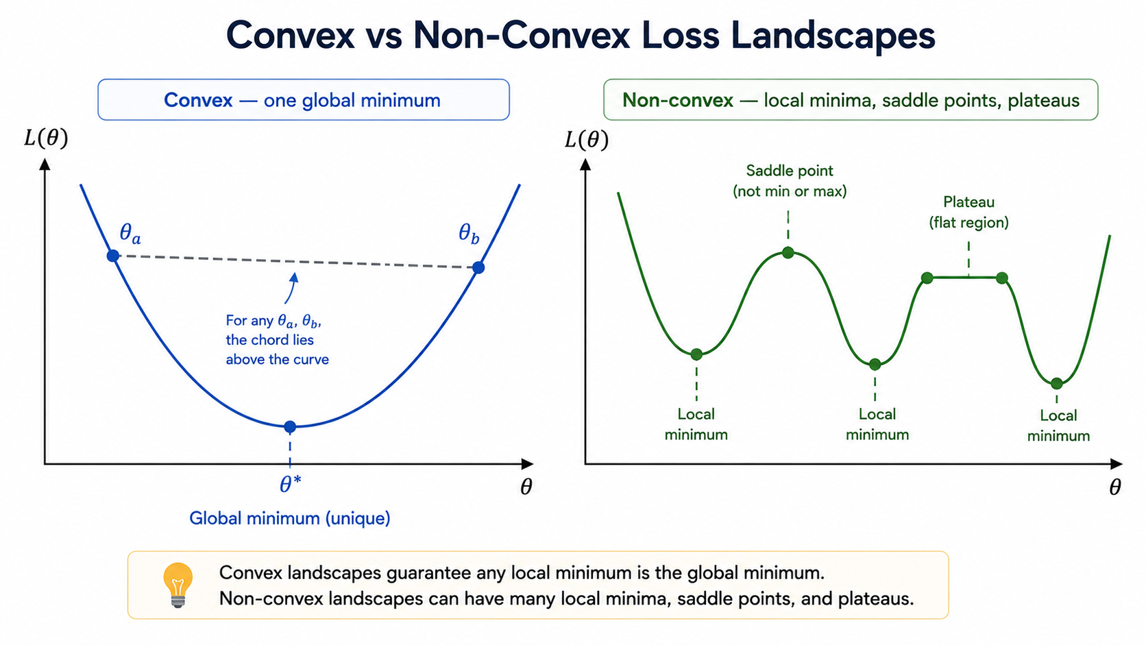
- ল্যান্ডস্কেপের আকার বা shape প্রচণ্ড গুরুত্বপূর্ণ। একটি মসৃণ বাটির মতো ল্যান্ডস্কেপ ধরে নিচে নামা খুব সহজ — যেকোনো জায়গা থেকে ঢাল বেয়ে নিচে নামতে থাকুন, আর আপনি শেষমেশ ওই একমাত্র তলানিতে গিয়ে পৌঁছবেনই। কিন্তু গর্ত, খাঁজ এবং সমতল মালভূমিতে ভরা একটি ল্যান্ডস্কেপে হাঁটা অনেক বেশি কঠিন, আর একটি আসল নিউরাল নেটওয়ার্ক ঠিক এই দ্বিতীয় ধরনের ল্যান্ডস্কেপই তৈরি করে।
এর পেছনের গণিত (The Math Behind It)
একটি অপ্টিমাইজেশন প্রবলেম হিসেবে ট্রেনিং (Training as an Optimization Problem)
যেখানে: হলো নেটওয়ার্কের ট্রেইন করার মতো বা trainable প্রতিটি প্যারামিটারের সংকলন (সব ওয়েটস এবং বায়াস একসাথে করে), হলো নেটওয়ার্কের ফাংশন, হলো প্রতিটি এক্সাম্পলের জন্য লস বা per-example loss (যেমন ক্রস-এন্ট্রপি, স্কয়ারড এরর, অথবা পরের চ্যাপ্টারে আলোচনা করা যেকোনো লস), এবং হলো পুরো ট্রেনিং সেটের ওপর গড়ের বা average লস।
পেছনের যুক্তি বা Intuition: এই একটি লাইনেই ট্রেনিংয়ের সম্পূর্ণ লক্ষ্য খুব নিখুঁতভাবে বলা আছে। এরপর আপনি যত অপ্টিমাইজারের দেখা পাবেন — যেমন সাধারণ গ্রেডিয়েন্ট ডিসেন্ট, মোমেন্টাম (Momentum), আরএমএসপ্রপ (RMSProp), অ্যাডাম (Adam) — সেগুলো সবই হলো হুবহু এই একই অনুসন্ধান বা search সমস্যাটির সমাধান করার এক একটি আলাদা স্ট্র্যাটেজি, যা আগেরটির চেয়ে বেশি নির্ভরযোগ্য বা দক্ষ।
এটি সরাসরি আগের চ্যাপ্টারগুলোর সাথে যুক্ত
পারসেপ্ট্রনের ভুল-শুধরানো বা mistake-driven আপডেট রুল এবং backpropagation-এর এরর সিগন্যাল — দুটোই নীরবে ঠিক এই কাজটাই করে আসছিল। Backpropagation মূলত — অর্থাৎ এই অবজেক্টিভটির গ্রেডিয়েন্ট — ক্যালকুলেট করে, আর এই চ্যাপ্টারটি আনুষ্ঠানিকভাবে বোঝায় যে একবার গ্রেডিয়েন্ট হাতে পাওয়ার পর সেটা দিয়ে আসলে কী করতে হয়।
কনভেক্স বনাম নন-কনভেক্স ল্যান্ডস্কেপ (Convex vs. Non-Convex Landscapes)
পেছনের যুক্তি বা Intuition: একটি ফাংশনকে তখনই কনভেক্স (convex) বলা হয়, যখন এর গ্রাফের ওপর যেকোনো দুটি বিন্দুকে যুক্ত করা একটি সরলরেখা কখনোই গ্রাফের নিচে নেমে যায় না। একটি মসৃণ বাটির কথা চিন্তা করুন: আপনি যেখান থেকেই শুরু করুন না কেন, ঢাল বেয়ে নিচে নামলে তা সবসময় একই এবং একমাত্র তলানিতে গিয়েই পৌঁছায়। কনভেক্সিটি আপনাকে ঠিক এই নিশ্চয়তা বা গ্যারান্টিটুকুই দেয়।
MLP লস সারফেসগুলো কনভেক্স নয়
হিডেন লেয়ার থাকা একটি Multi-Layer Perceptron-এর লস সারফেস (loss surface) সাধারণত নন-কনভেক্স (non-convex) হয়। তাত্ত্বিকভাবে গ্রেডিয়েন্ট ডিসেন্ট যে একমাত্র সেরা সমাধানটি খুঁজে পাবেই, এমন কোনো গ্যারান্টি নেই — এটি আটকে যেতে পারে। একটি সাধারণ লিনিয়ার মডেল এবং একটি MLP-এর মধ্যে এটাই হলো সবচেয়ে বড় পার্থক্য: শুধু একটি হিডেন লেয়ার ঢুকিয়ে দিন, আর আপনি একটি বন্ধুসুলভ বাটি আকৃতির ল্যান্ডস্কেপ হারিয়ে এমন একটি ল্যান্ডস্কেপ পাবেন যা এবড়োখেবড়ো এবং আগে থেকে ধারণা করার অযোগ্য। তবে বাস্তবে, আধুনিক বড় বড় নেটওয়ার্কের ওপর গবেষণায় দেখা গেছে যে, গ্রেডিয়েন্ট ডিসেন্ট যেসব ছোটখাটো গর্ত বা লোকাল মিনিমায় (local minima) গিয়ে পড়ে, সেগুলোও বেশ ভালোভাবেই কাজ বা জেনারেলাইজ (generalize) করতে পারে — বরং এর আসল বাধা হলো খারাপ লোকাল মিনিমা নয়, স্যাডল পয়েন্ট (saddle points)।
ক্রিটিকাল পয়েন্ট: মিনিমা, ম্যাক্সিমা এবং স্যাডল পয়েন্ট (Critical Points: Minima, Maxima, and Saddle Points)
একটি ক্রিটিকাল পয়েন্ট (critical point) হলো এমন যেকোনো পয়েন্ট যেখানে — অর্থাৎ ল্যান্ডস্কেপটি ওই মুহূর্তে সব দিকেই সমতল। কিন্তু সব সমতল জায়গাই এক রকম নয়:
| ধরন (Type) | দেখতে যেমন (What it looks like) | ট্রেনিংয়ের ওপর প্রভাব (Effect on training) |
|---|---|---|
| লোকাল মিনিমাম (Local minimum) | আশেপাশের সব পয়েন্টের চেয়ে নিচু | গ্রেডিয়েন্ট ডিসেন্ট এখানে এসে থামে এবং এখানেই থেকে যায় |
| লোকাল ম্যাক্সিমাম (Local maximum) | আশেপাশের সব পয়েন্টের চেয়ে উঁচু | অস্থিতিশীল — একটু নাড়াচাড়া করলেই এখান থেকে সরে যায় |
| স্যাডল পয়েন্ট (Saddle point) | কিছু দিকে ওপরে ওঠে, অন্য দিকে নিচে নামে | বেশিরভাগ দিকেই গ্রেডিয়েন্ট প্রায় শূন্যের কাছাকাছি চলে আসে, যা নেটওয়ার্ক পুরোপুরি আটকে না গেলেও ট্রেনিংকে দীর্ঘ সময়ের জন্য ধীর বা স্তব্ধ করে দেয় |
খারাপ মিনিমা নয়, স্যাডল পয়েন্টই হলো আসল ভিলেন
নিউরাল নেটওয়ার্কগুলো যে অত্যন্ত বিশাল ডাইমেনশনের বা মাত্রার স্পেসে (মিলিয়ন মিলিয়ন ওয়েটস নিয়ে) থাকে, সেখানে দেখা গেছে যে খারাপ লোকাল মিনিমার চেয়ে স্যাডল পয়েন্টের সংখ্যা বহুগুণ বেশি। একটি নেটওয়ার্ক হয়তো একটি প্রায়-সমতল স্যাডল অঞ্চলের ওপর দিয়ে হামাগুড়ি দিয়ে পার হতে লম্বা সময় লাগিয়ে দিতে পারে — এর কারণ এটা নয় যে সে সেখানে আটকে গেছে, বরং এর কারণ হলো প্রায় সব দিকেই ঢাল এতই সমতল যে সামনের দিকে আগানোটা যন্ত্রণাদায়কভাবে ধীর হয়ে যায়।
ব্যাচ, স্টোকাস্টিক এবং মিনি-ব্যাচ গ্রেডিয়েন্ট ডিসেন্ট (Batch, Stochastic, and Mini-Batch Gradient Descent)
আপডেটের মূল নিয়মটি বা রুলটি হলো , কিন্তু এর ভেতরেই একটি পছন্দ লুকিয়ে আছে: একটি ধাপ ফেলার আগে গ্রেডিয়েন্ট ক্যালকুলেট করার জন্য আপনি ঠিক কতটুকু ডেটা ব্যবহার করবেন?
| ভ্যারিয়েন্ট (Variant) | যেটার ওপর গ্রেডিয়েন্ট ক্যালকুলেট করা হয় | ট্রেড-অফ (Trade-off) |
|---|---|---|
| ব্যাচ গ্রেডিয়েন্ট ডিসেন্ট (Batch Gradient Descent) | পুরো ট্রেনিং সেট, প্রতিটি ধাপে | দিকটা খুব নিখুঁত, কিন্তু বড় ডেটাসেটে প্রতি আপডেট প্রচণ্ড ধীর |
| স্টোকাস্টিক গ্রেডিয়েন্ট ডিসেন্ট বা SGD (Stochastic Gradient Descent) | একটি মাত্র র্যান্ডম বা দৈব এক্সাম্পল | আপডেট খুব দ্রুত হয়, কিন্তু পথটা খুব নয়েজি এবং কাঁপুনিওয়ালা |
| মিনি-ব্যাচ গ্রেডিয়েন্ট ডিসেন্ট (Mini-Batch Gradient Descent) | একটি ছোট র্যান্ডম সাবসেট (যেমন 32-256 এক্সাম্পল) | বাস্তবে এটাই স্ট্যান্ডার্ড — এটি গতি এবং স্থিতিশীলতার মধ্যে দারুণ ভারসাম্য আনে |
এদের পূর্ণাঙ্গ তুলনা — কোডসহ এবং অ্যাডামের (Adam) মতো আধুনিক অপ্টিমাইজারের সাথে এগুলো কীভাবে কাজ করে তা নিয়ে — পরের চ্যাপ্টারে বিস্তারিত আলোচনা করা হয়েছে। আপাতত, মূল ধারণাটি হলো "গ্রেডিয়েন্ট ডিসেন্ট" কোনো একটি একক অ্যালগরিদম নয়, বরং এটি একটি ফ্যামিলি বা পরিবার।
লার্নিং রেট-এর ভূমিকা (The Role of the Learning Rate)
লার্নিং রেট হলো এখানকার সবচেয়ে প্রভাবশালী হাইপারপ্যারামিটার
যদি অনেক বড় হয়, তবে প্রতিটি ধাপ মিনিমামকে টপকে চলে যায় (overshoot), এবং ট্রেনিং পাগলের মতো এদিক-ওদিক ওঠানামা করতে বা একেবারেই দূরে সরে যেতে পারে (diverge)। আর যদি খুব ছোট হয়, তবে ট্রেনিং স্থিতিশীল হয় ঠিকই, কিন্তু এতটাই ধীরে এগোয় যে একটি ভালো সমাধানে পৌঁছাতে অনন্তকাল লেগে যেতে পারে, এবং এমন অবস্থায় কোনো সমতল বা স্যাডল অঞ্চলে দীর্ঘ সময়ের জন্য আটকে থাকার সম্ভাবনা অনেক বেড়ে যায়।
লার্নিং রেট এক্সপ্লোরার (Learning Rate Explorer)
একটি লার্নিং রেট বেছে নিন এবং একটি খুব সাধারণ বাটি-আকৃতির লস কার্ভের ওপর গ্রেডিয়েন্ট ডিসেন্টের ধাপগুলো দেখুন। রেট খুব ছোট, একদম পারফেক্ট, বা খুব বড় হলে কী হয় তা খেয়াল করুন।
Step 0
Try stepping through and watch how it behaves.
মোমেন্টাম এবং লার্নিং রেট শিডিউলিং: একটি ঝলক (A Glimpse of Momentum and Learning Rate Scheduling)
সাধারণ গ্রেডিয়েন্ট ডিসেন্টের একটি সীমাবদ্ধতা হলো এটির কোনো "স্মৃতি" নেই — প্রতিটি ধাপ শুধু বর্তমান গ্রেডিয়েন্টের ওপর নির্ভর করে, আগের ধাপগুলোর ওপর নয়। এর ফলে এটি সরু, প্রসারিত উপত্যকায় (যেমন উপরের দ্বিতীয় উদাহরণে) ধীরে ধীরে দুলতে দুলতে এগোয়।
সহজ কথায়: এখানে একটি "বেগ" বা velocity ভেক্টর যোগ করা হয়, যা আগের গ্রেডিয়েন্টগুলোর একটি ঘাটতিপ্রাপ্ত বা decaying গড় ধরে রাখে ( সাধারণত ০.৯ এর কাছাকাছি)। এটিকে একটি বলের গড়িয়ে পড়ার সাথে তুলনা করা যায়, যা শুধু স্থানীয় ঢালের ওপর নির্ভর না করে তার নিজস্ব জড়তা (momentum) বহন করে, যার ফলে সামঞ্জস্যপূর্ণ দিকে দ্রুত গতি বাড়ে আর বিপরীতমুখী দোলাচল কমে যায়।
লার্নিং রেট ট্রেনিং জুড়ে স্থির রাখারও দরকার নেই। একটি জনপ্রিয় কৌশল হলো লার্নিং রেট শিডিউলিং (learning rate scheduling), যেখানে ট্রেনিংয়ের শুরুতে বড় দিয়ে দ্রুত অগ্রসর হওয়া হয়, তারপর ধীরে ধীরে ছোট করা হয় যাতে শেষের দিকে মিনিমামের কাছাকাছি সূক্ষ্মভাবে (fine-tune) স্থির হওয়া যায়।
বিস্তারিত পরবর্তী চ্যাপ্টারে
মোমেন্টাম, RMSProp, এবং Adam-এর মতো অপ্টিমাইজার, এবং বিভিন্ন লার্নিং রেট শিডিউল, এই কোর্সের পরের অংশে সম্পূর্ণ বিস্তারিতভাবে আলোচনা করা হয়েছে। এখানে শুধু এটুকু বোঝাই যথেষ্ট যে সাধারণ গ্রেডিয়েন্ট ডিসেন্ট আপডেট রুল, θ ← θ − η∇L(θ), হলো একটি বড় পরিবারের সবচেয়ে সরল সদস্য, এবং বাকি সবগুলো এরই ওপর ভিত্তি করে তৈরি বুদ্ধিদীপ্ত সংযোজন।
হাতে-কলমে গাণিতিক উদাহরণ: গ্রেডিয়েন্ট ডিসেন্ট (Worked Example: Gradient Descent by Hand)
ধরা যাক, কে মিনিমাইজ করতে হবে, শুরু করা হচ্ছে থেকে এবং লার্নিং রেট দিয়ে।
প্রথম ধাপ — গ্রেডিয়েন্ট: ।
ইটারেশন ১:
ইটারেশন ২:
ইটারেশন ৩:
প্রতিটি ধাপের পর সংশোধনের বা কারেকশনের পরিমাণ ছোট হতে থাকে কারণ মিনিমামের দিকে এগোতে থাকে — অর্থাৎ গ্রেডিয়েন্ট নিজেই ছোট হতে থাকে, যেহেতু , হওয়ার সাথে সাথে শূন্যের দিকে এগোয়। এভাবেই চলতে থাকলে, একসময় -এর দিকে কনভার্জ করে বা স্থির হয়, যা বীজগণিত বা অ্যালজেবরা দিয়েও মিলে যায়: , এবং নিশ্চিত করে যে এটি আসলেই একটি মিনিমাম, ম্যাক্সিমাম নয়।
লস কার্ভ কীভাবে পড়তে হয় (Reading a loss curve)
ইটারেশন নম্বরের বিপরীতে লস প্লট করে দেখাটা পুরো Deep Learning-এ আপনার অন্যতম সেরা অভ্যাস। লস একটানা কমতে থাকলে এবং ধীরে ধীরে সমতল হতে থাকলে বুঝবেন কনভার্জেন্স স্বাস্থ্যকর। পাগলের মতো ওঠানামা করলে বুঝবেন লার্নিং রেট খুব বেশি। আর খুব বিরক্তিকর ধীরগতিতে, প্রায়-সমতল অবস্থায় কমতে থাকলে বুঝবেন লার্নিং রেট খুব কম।
দ্বিতীয় উদাহরণ — দুটি প্যারামিটার একসাথে (Gradient Descent in Two Dimensions): এবার ধরা যাক একটি এমন লস আছে যা দুটি প্যারামিটারের ওপর নির্ভর করে: L(w1,w2) = w1^2 + 4w2^2। এটি আসলে ক্যালকুলাস চ্যাপ্টারে দেখা ImagePlaceholder-এর উপবৃত্তাকার (elliptical) বাটি-আকৃতির লসেরই একটি সংস্করণ। শুরু করা হচ্ছে (w1,w2) = (2, 1) থেকে, লার্নিং রেট η = 0.1 দিয়ে।
গ্রেডিয়েন্ট: ∂L/∂w1 = 2w1, ∂L/∂w2 = 8w2।
ইটারেশন ১: গ্রেডিয়েন্ট (4, 8)-এ, তাই (w1,w2) = (2 - 0.1(4), 1 - 0.1(8)) = (1.6, 0.2)
ইটারেশন ২: গ্রেডিয়েন্ট (3.2, 1.6)-এ, তাই (w1,w2) = (1.6 - 0.1(3.2), 0.2 - 0.1(1.6)) = (1.28, 0.04)
খেয়াল করুন একটি গুরুত্বপূর্ণ ব্যাপার: w2 (যার গ্রেডিয়েন্টের সহগ 8, অনেক বড়) w1-এর (সহগ 2) চেয়ে অনেক দ্রুত মিনিমামের কাছে পৌঁছে যাচ্ছে। এটিই হলো একটি "প্রসারিত" বা elongated বাটি-আকৃতির লস ল্যান্ডস্কেপের বৈশিষ্ট্য, যেখানে বিভিন্ন দিকে বক্রতা (curvature) ভিন্ন ভিন্ন হয়। এই ধরনের ভিন্ন ভিন্ন বক্রতার সমস্যাটিই মোমেন্টাম এবং অ্যাডাম-এর মতো আধুনিক অপ্টিমাইজারের মূল অনুপ্রেরণা, যা পরের চ্যাপ্টারে বিস্তারিত আলোচনা করা হয়েছে।
Implementation
python
এটি ঠিক হাতে-কলমে করা উদাহরণের মতোই কাজ করে: প্রতিটি ইটারেশন বর্তমান পয়েন্টে গ্রেডিয়েন্ট নতুন করে ক্যালকুলেট করে এবং তার উল্টোদিকে একটি আনুপাতিক ধাপ ফেলে। কোডটি রান করলে দেখা যায় যে theta প্রায় 2.0-এর দিকে কনভার্জ করে, যা গাণিতিক সমাধানের সাথে পুরোপুরি মিলে যায়।
মূল বিষয়গুলো (Key Takeaways)
Key Takeaways
- একটি নেটওয়ার্ক ট্রেন করা মূলত একটি অনুসন্ধান বা search: এমন একটি খুঁজে বের করা যা -কে মিনিমাইজ বা সবচেয়ে ছোট করে।
- কনভেক্স লস সারফেসগুলোর একটিমাত্র গ্লোবাল মিনিমাম থাকে যা গ্রেডিয়েন্ট ডিসেন্ট দিয়ে নির্ভরযোগ্যভাবে পৌঁছানো সম্ভব; কিন্তু MLP-এর লস সারফেসগুলো সাধারণত নন-কনভেক্স হয়।
- বিশাল ডাইমেনশনের নন-কনভেক্স অপ্টিমাইজেশনের ক্ষেত্রে, খারাপ লোকাল মিনিমার চেয়ে স্যাডল পয়েন্টগুলো ট্রেনিংকে বেশি বাধা দেয়।
- ব্যাচ, স্টোকাস্টিক এবং মিনি-ব্যাচ গ্রেডিয়েন্ট ডিসেন্টগুলো মূলত আপডেটের পেছনে লাগা কম্পিউটেশনাল খরচের বিনিময়ে গ্রেডিয়েন্টের নিখুঁত হওয়া বা না হওয়ার মধ্যে একটি ট্রেড-অফ।
- লার্নিং রেট কনভার্জেন্সের স্থিতিশীলতা এবং গতি — দুটোই নিয়ন্ত্রণ করে। খুব বেশি হলে ডাইভার্জ বা দূরে সরে যায়, আর খুব কম হলে শামুকের মতো এগোয়।
সাধারণ ভুল ধারণা (Common Mistakes)
গ্রেডিয়েন্ট ডিসেন্ট সবসময় সেরা সমাধানটিই খুঁজে পাবে, এমনটা ধরে নেওয়া
এই গ্যারান্টিটুকু শুধুমাত্র কনভেক্স ফাংশনের জন্যই সত্য। একটি MLP-এর লস সারফেস প্রায় কখনোই কনভেক্স হয় না, তাই "লস কমা বন্ধ হয়ে গেছে" মানেই যে "আমরা সম্ভাব্য সেরা ওয়েটস পেয়ে গেছি" তা কিন্তু নয় — এর মানে এমনও হতে পারে যে ট্রেনিং কোনো স্যাডল পয়েন্ট বা মাঝারি মানের লোকাল মিনিমায় আটকে গেছে।
লার্নিং রেট-কে খুব সাধারণ বা কম গুরুত্বপূর্ণ কিছু বলে ধরে নেওয়া
যেকোনো টিউটোরিয়ালে যা দেওয়া থাকে, সেই ডিফল্ট লার্নিং রেটটাই রেখে দেওয়াটা খুব প্রলুব্ধকর। কিন্তু বাস্তবে, ট্রেনিং আদৌ সফল হবে কি না, তার পেছনে বেশিরভাগ সময়ে এই একটিমাত্র হাইপারপ্যারামিটারই দায়ী থাকে — নতুন কোনো ভ্যালু চেষ্টা করে দেখার সময় সবসময় লস কার্ভের দিকে কড়া নজর রাখুন।
মিনি-ব্যাচ সাইজকে গুরুত্বহীন হাইপারপ্যারামিটার মনে করা
ব্যাচ সাইজ শুধু ট্রেনিং স্পিডকেই প্রভাবিত করে না, এটি গ্রেডিয়েন্ট এস্টিমেটের নয়েজের পরিমাণও নিয়ন্ত্রণ করে। খুব বড় ব্যাচ সাইজ মসৃণ কিন্তু কম explorative গ্রেডিয়েন্ট দেয়, যা কখনো কখনো একটি বাজে শার্প (sharp) মিনিমায় আটকে যেতে পারে; খুব ছোট ব্যাচ সাইজ নয়েজি গ্রেডিয়েন্ট দেয়, যা মাঝে মাঝে সহায়ক (স্যাডল পয়েন্ট থেকে বের হতে) আবার মাঝে মাঝে ক্ষতিকর (কনভার্জেন্স অস্থিতিশীল করে) হতে পারে।
মোমেন্টামকে লার্নিং রেটের বিকল্প ভেবে নেওয়া
মোমেন্টাম লার্নিং রেট বেছে নেওয়ার প্রয়োজনীয়তা দূর করে না — এটি শুধু আপডেটগুলোকে মসৃণ করে এবং সামঞ্জস্যপূর্ণ দিকে গতি বাড়ায়। ভুল লার্নিং রেটের সাথে মোমেন্টাম ব্যবহার করলে সমস্যা কমার বদলে বরং বাড়তেও পারে, কারণ জমে থাকা ভেলোসিটি একটি খারাপ দিকে আরও জোরে ধাক্কা দিতে পারে।
ইন্টারভিউ কর্নার (Interview Corner)
Quick Check
বাস্তবে এটি কোথায় দেখা যায় (Where This Shows Up in Practice)
আপনি জীবনে যত ট্রেনিং রান (training run) চালু করবেন — তা সে দুই-লেয়ারের MLP হোক বা এক-বিলিয়ন-প্যারামিটারের ল্যাঙ্গুয়েজ মডেলই হোক — তার প্রতিটিই ঠিক এই অনুসন্ধান সমস্যাটিরই বা search problem-এর এক একটি উদাহরণ। এই অনুসন্ধান চালানোর জন্য ব্যবহৃত সুনির্দিষ্ট অ্যালগরিদমটি (যেমন সাধারণ গ্রেডিয়েন্ট ডিসেন্ট, মোমেন্টাম, অ্যাডাম এবং আরও অনেক কিছু) পরের দুটি চ্যাপ্টারের মূল বিষয়, কিন্তু এর ভেতরের মূল লক্ষ্যটি কখনোই বদলায় না: গ্রেডিয়েন্টের সাহায্যে এমন একটি খুঁজে বের করা যা ধাপে ধাপে -কে যতটা সম্ভব ছোট করে তোলে।