Chapter 17 of 25
Optimizers
Smarter ways to walk downhill
22 min read
Created ২ আগ, ২০২৬
ভূমিকা (Motivation)
সাধারণ গ্রেডিয়েন্ট ডিসেন্ট (gradient descent) ঠিকমতোই কাজ করে, এই অর্থে যে এটি গ্যারান্টি দেয় যে সে নিচের দিকেই নামবে। কিন্তু "শেষ পর্যন্ত গন্তব্যে পৌঁছাবে" আর "যৌক্তিক বা ঠিকঠাক সময়ের মধ্যে পৌঁছাবে" — এই দুটি কথার মধ্যে আকাশ-পাতাল তফাত। বাস্তবের লস সারফেসগুলোতে সরু উপত্যকা (ravines), বিভিন্ন দিকে পাগলের মতো ওঠানামা করা সেনসিটিভিটি (sensitivities), এবং দীর্ঘ, প্রায় সমতল মালভূমি (plateaus) থাকে — আর সাধারণ গ্রেডিয়েন্ট ডিসেন্ট, যার কাছে শুধু বর্তমান গ্রেডিয়েন্ট এবং একটি ফিক্সড লার্নিং রেট ছাড়া আর কিছুই নেই, সে এগুলো খুব বাজেভাবে সামলায়। এটি সরু উপত্যকার দেয়ালে বাড়ি খেয়ে এদিক-ওদিক ধাক্কা খায়, সমতল মালভূমিতে শামুকের মতো এগোয়, আর এর একটামাত্র লার্নিং রেটকে একই সাথে প্রতিটি প্যারামিটারের জন্য ঠিক হতে হয়, যা প্রায় অসম্ভব।
এই চ্যাপ্টারের প্রতিটি অপ্টিমাইজার (optimizer) তৈরি হয়েছে তার ঠিক আগেরটির একটি নির্দিষ্ট দুর্বলতা ঠিক করার জন্য। ফর্মুলা মুখস্থ না করে, এই ভুলগুলো কীভাবে ধাপে ধাপে ঠিক করা হয়েছে তা বোঝাটাই হলো পুরো অপ্টিমাইজার ফ্যামিলিকে সহজে আয়ত্ত করার চাবিকাঠি। আর ঠিক এ কারণেই অ্যাডাম (Adam), যে অপ্টিমাইজারটি প্রায় সবাই চোখ বন্ধ করে ব্যবহার করে, তার চেহারাটা ঠিক অমন।
একটি বাস্তব জীবনের উদাহরণ (A Real-Life Scenario)
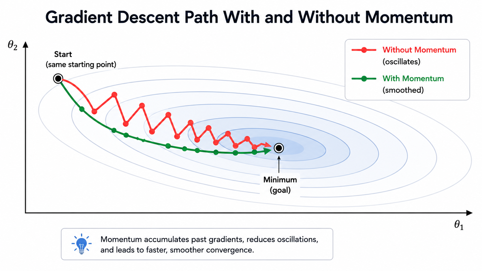
ভাবুন তো, কেউ একজন একটি খাড়া, সরু পাহাড়ি উপত্যকা বেয়ে একদম নিচের একটি নদীর দিকে নামছে। সে যদি সবসময় শুধু ঠিক সেই দিকেই পা ফেলে যেদিকে তার পায়ের ঠিক নিচের মাটিটা ঢালু, তবে সে সরু উপত্যকার এ-দেয়াল থেকে ও-দেয়ালে পাগলের মতো জিগজ্যাগ (zigzag) করতে করতে নদীর দিকে খুব ধীরগতিতে এগোবে, যদিও টেকনিক্যালি তার প্রতিটি পদক্ষেপই "নিচের দিকে"। এর বদলে একজন অভিজ্ঞ হাইকার বা পর্বতারোহী তার আগের হাঁটার দিকের কিছু মোমেন্টাম বা ভরবেগ (momentum) ধরে রাখে, যা ওই জিগজ্যাগ পথটাকে মসৃণ করে একটি সরাসরি সামনের দিকের পথে পরিণত করে — আর সে যদি এমন পথ বেছে নিতে শুরু করে যেখানে আগে থেকেই মাটিটা কিছুটা মসৃণভাবে ঢালু ছিল (খাড়া এবং এবড়োখেবড়ো রাস্তার বদলে), তবে সে আরও অনেক দ্রুত এবং বিনা পরিশ্রমে নিচে নামতে পারবে।
এটাই হলো এই চ্যাপ্টারের পুরো গল্প: মোমেন্টাম (momentum) ওই জিগজ্যাগ পথটাকে মসৃণ করে, আর প্রতিটি প্যারামিটারের জন্য আলাদা বা অ্যাডাপ্টিভ (adaptive) লার্নিং রেটগুলো খাড়া ও কাঁপুনিওয়ালা দিকগুলোর বদলে অপেক্ষাকৃত মসৃণ এবং তথ্যবহুল দিকগুলোকে বেশি গুরুত্ব দেয়।
মূল ধারণা তৈরি করা (Building the Intuition)
- এখানকার প্রতিটি অপ্টিমাইজার একই কঙ্কাল বা কাঠামোর ওপর দাঁড়িয়ে আছে: একটি গ্রেডিয়েন্ট ক্যালকুলেট করুন, তারপর সেই গ্রেডিয়েন্টের কোনো একটি ফাংশন দিয়ে প্যারামিটারগুলো আপডেট বা অ্যাডজাস্ট করুন। এদের মধ্যে পার্থক্য শুধু একটাই — এরা প্রত্যেকে আলাদা আলাদা বাড়তি তথ্য জমা রাখে এবং ব্যবহার করে।
- মোমেন্টাম (Momentum)-ভিত্তিক মেথডগুলো বা পদ্ধতিগুলো আগের গ্রেডিয়েন্টগুলোর একটি রানিং অ্যাভারেজ বা গড় মনে রাখে, যা ওই নয়েজি (noisy) জিগজ্যাগ পথটাকে মসৃণ করে।
- অ্যাডাপ্টিভ (Adaptive) মেথডগুলো (AdaGrad, RMSProp, Adam) প্রতিটি আলাদা প্যারামিটারকে তার নিজস্ব কার্যকর লার্নিং রেট দেয়, যা নির্ভর করে ওই প্যারামিটারের গ্রেডিয়েন্টগুলো অতীতে কতটা বড় বা ছোট ছিল তার ওপর।
- অ্যাডাম (Adam) খুব সিম্পলভাবে এই দুটো ধারণাকেই — অর্থাৎ মোমেন্টামের মসৃণ করার ক্ষমতা এবং RMSProp-এর প্যারামিটার অনুযায়ী অ্যাডাপ্টিভ হওয়ার ক্ষমতা — একটি অপ্টিমাইজারের ভেতর এক করে দেয়, আর ঠিক এ কারণেই এটি আজ সবার ডিফল্ট পছন্দ হিসেবে রাজত্ব করছে।
একটি খুব সহজ মানসিক মডেল
প্রতিটি অপ্টিমাইজারকে দুটি প্রশ্নের উত্তর হিসেবে দেখুন: (১) কোন দিকে যাব — শুধু বর্তমান গ্রেডিয়েন্ট, নাকি অতীতের গ্রেডিয়েন্টগুলোর একটি মসৃণ করা গড়? আর (২) কতটুকু যাব — একটিমাত্র গ্লোবাল লার্নিং রেট, নাকি প্রতিটি প্যারামিটারের নিজস্ব ইতিহাসের ওপর ভিত্তি করে আলাদা আলাদা স্টেপ সাইজ? SGD দুটি প্রশ্নেরই সবচেয়ে সহজ উত্তর দেয়; Adam দুটোরই সবচেয়ে পরিশীলিত উত্তর দেয়।
এর পেছনের গণিত (The Math Behind It)
ব্যাচ, স্টোকাস্টিক এবং মিনি-ব্যাচ গ্রেডিয়েন্ট ডিসেন্ট (Batch, Stochastic, and Mini-Batch Gradient Descent)
ব্যাচ গ্রেডিয়েন্ট ডিসেন্ট (Batch Gradient Descent):
স্টোকাস্টিক গ্রেডিয়েন্ট ডিসেন্ট (Stochastic Gradient Descent / SGD):
মিনি-ব্যাচ গ্রেডিয়েন্ট ডিসেন্ট (Mini-Batch Gradient Descent):
যেখানে: হলো পুরো ডেটাসেটের সাইজ এবং হলো মিনি-ব্যাচ সাইজ (সাধারণত 32, 64, 128, বা 256)।
| ভ্যারিয়েন্ট (Variant) | সুবিধাসমূহ (Advantages) | অসুবিধাসমূহ (Disadvantages) |
|---|---|---|
| ব্যাচ GD (Batch GD) | স্থিতিশীল, নিখুঁত গ্রেডিয়েন্টের দিক | বড় ডেটাসেটে প্রতি আপডেট প্রচণ্ড ধীর; পুরো ডেটাসেটকে মেমোরিতে রাখতে হয় |
| SGD | খুব দ্রুত আপডেট হয়; এর নয়েজ অগভীর মিনিমা/স্যাডল পয়েন্ট থেকে বের হতে সাহায্য করতে পারে | গ্রেডিয়েন্টের অনুমান খুব নয়েজি বা ভুল হতে পারে; লস কার্ভ খুব বেশি ওঠানামা করে; হার্ডওয়্যারের বাজে ব্যবহার |
| মিনি-ব্যাচ GD (Mini-Batch GD) | গতি এবং স্থিতিশীলতার দারুণ ভারসাম্য; ভেক্টরাইজড/GPU হার্ডওয়্যারে খুব দক্ষ | একটি ব্যাচ সাইজ বেছে নিতে হয় (যা একটি অতিরিক্ত হাইপারপ্যারামিটার) |
একটি টার্মিনোলজি ওভারলোড যা জানা থাকা ভালো
বাস্তবে মিনি-ব্যাচ গ্রেডিয়েন্ট ডিসেন্ট প্রায় সব জায়গাতেই ব্যবহৃত হয়। কাজ করার সময় মানুষ যখন কথায় কথায় "SGD" বলে, তখন তারা খুব সম্ভবত মিনি-ব্যাচ গ্রেডিয়েন্ট ডিসেন্ট, অথবা নিচে দেওয়া মোমেন্টাম/অ্যাডাপ্টিভ ভ্যারিয়েন্টগুলোর কোনো একটিকেই বোঝায় — পেপার বা ফ্রেমওয়ার্ক পড়ার সময় শব্দের এই কমন ওভারলোডের বা ব্যাপ্তির বিষয়ে খেয়াল রাখবেন।
মোমেন্টাম (Momentum)
যেখানে: হলো "ভেলোসিটি বা বেগ" — যা আগের গ্রেডিয়েন্টগুলোর একটি এক্সপোনেনশিয়ালি ওয়েটেড মুভিং অ্যাভারেজ (exponentially weighted moving average) — এবং (সাধারণত 0.9) ঠিক করে দেয় যে অতীতের কতটুকু গ্রেডিয়েন্ট মনে রাখা হবে।
পেছনের যুক্তি বা Intuition: ভাবুন একটি বল লস সারফেস বেয়ে নিচে গড়িয়ে পড়ছে। শুধু বর্তমান গ্রেডিয়েন্টের ওপর নির্ভর করার বদলে, মোমেন্টাম এমন একটি বেগ বা ভেলোসিটি জমা করে যা গ্রেডিয়েন্টের নয়েজি বা এদিক-ওদিক হওয়া দিকগুলোকে মসৃণ করে দেয় এবং অপ্টিমাইজারকে সমতল অঞ্চল বা অগভীর লোকাল মিনিমার ওপর দিয়ে চলতে সাহায্য করে, ঠিক যেমনটা ফিজিক্যাল মোমেন্টাম বা বাস্তব জীবনের ভরবেগ একটি গড়িয়ে পড়া বলকে ছোটখাটো গর্ত পার হতে সাহায্য করে।
নেস্টেরভ অ্যাক্সিলারেটেড গ্রেডিয়েন্ট বা NAG (Nesterov Accelerated Gradient)
স্ট্যান্ডার্ড মোমেন্টাম বর্তমান পজিশনে বা অবস্থানে গ্রেডিয়েন্ট ক্যালকুলেট করে, তারপর জমা হওয়া ভেলোসিটি প্রয়োগ করে। কিন্তু নেস্টেরভ (Nesterov) মোমেন্টাম ঠিক উল্টোটা করে: এটি ভেলোসিটি যেদিকে যেতে চলেছে ঠিক সেই পজিশনে গ্রেডিয়েন্ট ক্যালকুলেট করে — যাকে বলে একটি "লুক-অ্যাহেড (look-ahead)" বা সামনে তাকানোর ধাপ — যা অপ্টিমাইজারকে মিনিমাম টপকে যাওয়ার বা ওভারশুট (overshoot) করার আগেই ভুল শুধরে নেওয়ার সুযোগ দেয়, পরে নয়। এটি সাধারণত সাধারণ মোমেন্টামের চেয়ে অনেক দ্রুত এবং স্থিতিশীল কনভার্জেন্স দেয়।
অ্যাডাগ্র্যাড (AdaGrad)
যেখানে: প্রতিটি প্যারামিটারের জন্য আলাদাভাবে স্কয়ারড গ্রেডিয়েন্টের যোগফল জমা করে, এবং হলো একটি ছোট কনস্ট্যান্ট বা ধ্রুবক যা শূন্য দিয়ে ভাগ হওয়া আটকায়।
পেছনের যুক্তি বা Intuition: অ্যাডাগ্র্যাড প্রতিটি প্যারামিটারকে তার নিজস্ব অ্যাডাপ্টিভ লার্নিং রেট দেয় — যেসব প্যারামিটার অতীতে খুব বড় বড় গ্রেডিয়েন্ট পেয়েছে, তাদের কার্যকর লার্নিং রেট ছোট করে দেওয়া হয়, আর যেসব প্যারামিটার ছোট বা মাঝে মাঝে গ্রেডিয়েন্ট পেয়েছে, তাদের কার্যকর লার্নিং রেট তুলনামূলকভাবে বড় রাখা হয়। স্পার্স ফিচারের (sparse features) ক্ষেত্রে, যেগুলো খুব কম আপডেট হয়, সেখানে এটি খুব কাজে লাগে।
অ্যাডাগ্র্যাডের মারাত্মক একটি ত্রুটি (AdaGrad's fatal flaw)
যেহেতু সবসময় শুধু জমাই করতে থাকে এবং কখনোই কমে না, তাই অ্যাডাগ্র্যাডের কার্যকর লার্নিং রেট ট্রেনিং চলাকালীন ক্রমাগত কমতেই থাকে এবং একসময় তা এতটাই ছোট হয়ে যেতে পারে যে কার্যকরভাবে শেখা পুরোপুরি বন্ধ হয়ে যায়, এমনকি মডেলটি কনভার্জ করার আগেই। ঠিক এই সমস্যাটিই সরাসরি RMSProp এবং Adam-এর জন্ম দিয়েছে।
আরএমএসপ্রপ (RMSProp)
RMSProp, অ্যাডাগ্র্যাডের মূল সমস্যাটি সমাধান করে: এটি সবসময় বাড়তে থাকা যোগফল -কে একটি এক্সপোনেনশিয়ালি ডিকেয়িং (exponentially decaying) বা ক্রমশ কমতে থাকা মুভিং অ্যাভারেজ দিয়ে বদলে দেয় (যার কমার হার নিয়ন্ত্রণ করে , সাধারণত 0.9)। যেহেতু পুরোনো গ্রেডিয়েন্টগুলো ধীরে ধীরে "ভুলে যাওয়া" হয়, তাই কার্যকর লার্নিং রেট আর কমতে কমতে শূন্যতে গিয়ে ঠেকে না, এবং ট্রেনিং পুরো সময় জুড়েই নিজেকে মানিয়ে নিতে পারে বা অ্যাডাপ্ট করতে পারে।
অ্যাডাডেল্টা (AdaDelta)
অ্যাডাডেল্টা, RMSProp-কে আরও এক ধাপ এগিয়ে নিয়ে যায়: এটি শুধু গ্রেডিয়েন্ট নয়, বরং আগের প্যারামিটার আপডেটগুলোর একটি মুভিং অ্যাভারেজও মেনটেইন করে, এবং প্রতিটি আপডেটের সাইজ বা আকার ঠিক করতে এই দুটি মুভিং অ্যাভারেজের অনুপাত বা রেশিও (ratio) ব্যবহার করে। এর ফলে নিজে থেকে আর কোনো গ্লোবাল লার্নিং রেট ঠিক করে দেওয়ার দরকারই পড়ে না — তাত্ত্বিকভাবে এটি দারুণ একটি বৈশিষ্ট্য, যদিও বাস্তবে অ্যাডামের শক্তিশালী পারফরম্যান্স এবং এর অনেক সহজ ও স্বজ্ঞাত হাইপারপ্যারামিটারের কারণে অ্যাডামই এখন সবচেয়ে বেশি জনপ্রিয়।
অ্যাডাম (Adam / Adaptive Moment Estimation)
অ্যাডাম মোমেন্টামের আইডিয়া (গ্রেডিয়েন্টগুলোর একটি মুভিং অ্যাভারেজ রাখা) এবং RMSProp-এর আইডিয়াকে (স্কয়ারড গ্রেডিয়েন্টগুলোর একটি মুভিং অ্যাভারেজ রাখা) একটিমাত্র অপ্টিমাইজারের ভেতর এক করে ফেলে — আর এভাবেই এটি MLP-সহ আজকের বেশিরভাগ আধুনিক নিউরাল নেটওয়ার্ক ট্রেন করার ক্ষেত্রে ডিফল্ট পছন্দ হয়ে উঠেছে।
যেখানে: ; এর সাধারণ ডিফল্ট মানগুলো হলো , , ।
বায়াস কারেকশন কেন দরকার: যেহেতু , তাই raw মুভিং অ্যাভারেজগুলো ট্রেনিংয়ের প্রথম কয়েক ধাপে, যখন খুব ছোট থাকে, শূন্যের দিকে বেশ বায়াসড (biased) বা হেলে থাকে। এবং দিয়ে ভাগ করলে এই ইনিশিয়ালাইজেশন বায়াসটি হুবহু ঠিক হয়ে যায়, যা ট্রেনিংয়ের শুরুর দিকে খুব গুরুত্বপূর্ণ।
ইন্টারভিউয়ের খুব সাধারণ একটি প্রশ্ন
"অ্যাডাম এত জনপ্রিয় কেন?" উত্তরে বলুন যে, এটি নয়েজি গ্রেডিয়েন্টকে মসৃণ করতে মোমেন্টাম এবং প্রতিটি প্যারামিটারের জন্য আলাদা লার্নিং রেট দিতে RMSProp-এর আইডিয়াগুলোকে এক করেছে, সেই সাথে ট্রেনিংয়ের শুরুতে স্থিতিশীলতার জন্য বায়াস কারেকশন যোগ করেছে, এবং এটি খুব সামান্য হাইপারপ্যারামিটার টিউনিং করেই অসংখ্য সমস্যার ওপর খুব ভালো কাজ করে — অর্থাৎ এটি একটি খুব শক্তিশালী ডিফল্ট অপ্টিমাইজার।
অ্যাডাম-ডাব্লিউ (AdamW)
স্ট্যান্ডার্ড অ্যাডামকে যখন লসের ভেতরে একটি অতিরিক্ত পেনাল্টি টার্ম হিসেবে যোগ করা L2 রেগুলারাইজেশনের (L2 regularization) সাথে ব্যবহার করা হয়, তখন এটি অ্যাডামের অ্যাডাপ্টিভ লার্নিং রেটের সাথে খুব বাজেভাবে রিয়্যাক্ট করে — এর ফলে যেসব প্যারামিটারে বড় গ্রেডিয়েন্ট জমা হয়েছে, তাদের জন্য রেগুলারাইজেশন বেশ দুর্বল হয়ে পড়ে। AdamW এই সমস্যার সমাধান করে ওয়েট ডিকে-কে (weight decay) গ্রেডিয়েন্ট ক্যালকুলেশনের ভেতর না ঢুকিয়ে বরং একটি আলাদা এবং সরাসরি ধাপ হিসেবে প্রয়োগ করে (), যা একে অ্যাডামের অ্যাডাপ্টিভ স্কেলিং থেকে পুরোপুরি আলাদা করে দেয়। বেশিরভাগ আধুনিক Deep Learning-এর কাজগুলোতে, বিশেষ করে ট্রান্সফর্মার-ভিত্তিক (Transformer-based) মডেলগুলোতে, এখন AdamW-ই হলো স্ট্যান্ডার্ড পছন্দ।
ন্যাডাম এবং লায়ন (সংক্ষিপ্ত নোট) (Nadam and Lion)
ন্যাডাম (Nadam / Nesterov-accelerated Adam) নেস্টেরভ মোমেন্টামে ব্যবহৃত লুক-অ্যাহেড (look-ahead) আইডিয়াটিকে অ্যাডামের মোমেন্টাম টার্মের ওপর প্রয়োগ করে, যার লক্ষ্য হলো অ্যাডামের অ্যাডাপ্টিভ লার্নিং রেট এবং নেস্টেরভের উন্নত কনভার্জেন্সকে একসাথে মিলিয়ে দেওয়া। এটি সাধারণত স্ট্যান্ডার্ড অ্যাডামের মতোই, বা তার চেয়ে সামান্য ভালো পারফর্ম করে।
লায়ন (Lion / EvoLved Sign Momentum) হলো অপেক্ষাকৃত নতুন একটি অপ্টিমাইজার, যা অপ্টিমাইজারের ডিজাইনের ওপর স্বয়ংক্রিয় সার্চ করে আবিষ্কার করা হয়েছে। এটি প্যারামিটার আপডেট করতে মোমেন্টাম-দিয়ে-মসৃণ-করা একটি গ্রেডিয়েন্টের শুধু সাইন (sign) বা চিহ্ন ব্যবহার করে — অর্থাৎ গ্রেডিয়েন্টের raw মানের ওপর নির্ভর করে না — এবং একে AdamW-এর মতো ডিকাপলড ওয়েট ডিকে-র (decoupled weight decay) সাথে মিলিয়ে নেয়। এটি অ্যাডামের চেয়ে বেশ কম মেমরি ব্যবহার করে, কারণ এটি দ্বিতীয় কোনো মোমেন্ট (second moment) ট্র্যাক করে না, এবং এটি বড় বড় ভিশন (vision) ও ল্যাঙ্গুয়েজ মডেলে (language models) বেশ ভালো রেজাল্ট দেখিয়েছে। তবে, এটি Deep Learning-এর সমস্ত কাজ জুড়ে অ্যাডাম বা AdamW-এর মতো অতটা পরীক্ষিত নয়।
গ্রেডিয়েন্ট ক্লিপিং (Gradient Clipping)
মোমেন্টাম বা অ্যাডাপ্টিভ মেথড কোনোটিই একটি ভয়ংকর সমস্যা থেকে সরাসরি রক্ষা করে না: মাঝে মাঝে কোনো একটি নির্দিষ্ট মিনি-ব্যাচে (বিশেষ করে RNN-এর মতো রিকারেন্ট আর্কিটেকচারে, অথবা লস সারফেসের কোনো খাড়া "দেয়াল বা cliff"-এর কাছে) গ্রেডিয়েন্ট হঠাৎ অস্বাভাবিকভাবে বিশাল হয়ে যেতে পারে, যার ফলে একটি মাত্র আপডেটই ওয়েটগুলোকে সম্পূর্ণ অকেজো কোনো মানে ঠেলে দিতে পারে (এক ধাপেই NaN বা inf)।
যেখানে: হলো একটি থ্রেশহোল্ড বা সীমা (সাধারণত ১ থেকে ৫-এর মধ্যে), এবং হলো সমস্ত প্যারামিটারের গ্রেডিয়েন্ট একসাথে নিয়ে ক্যালকুলেট করা গ্লোবাল নর্ম।
সহজ কথায়: গ্রেডিয়েন্টের দিক অপরিবর্তিত থাকে, শুধু এর ম্যাগনিটিউড বা আকার -এর বেশি হলে তাকে সংকুচিত করে ঠিক -তে নামিয়ে আনা হয়। এটি অপ্টিমাইজারকে ঠিক দিকেই এগোতে দেয়, কিন্তু কোনো একটি বিপর্যয়কর বড় ধাপ নিতে বাধা দেয়।
কখন গ্রেডিয়েন্ট ক্লিপিং লাগে
সাধারণ MLP-তে (ফুললি কানেক্টেড, মাঝারি গভীরতার) গ্রেডিয়েন্ট এক্সপ্লোশন খুব একটা সাধারণ সমস্যা নয়, তবে RNN, খুব গভীর নেটওয়ার্ক, অথবা খুব বড় লার্নিং রেটের সাথে এটি খুবই প্রাসঙ্গিক। যদি ট্রেনিংয়ের লস হঠাৎ NaN হয়ে যায় বা কোনো ব্যাখ্যাহীন স্পাইক (spike) দেখা যায়, তবে গ্রেডিয়েন্ট ক্লিপিং যোগ করাটাই প্রথম চেক করার মতো একটি সমাধান।
হাতে-কলমে সংখ্যাগত তুলনা: SGD বনাম মোমেন্টাম (Worked Numeric Comparison)
আগের সরু-উপত্যকা লসটি নিয়ে প্রথম ধাপ হাতে-কলমে ট্রেস করা যাক, যেখানে ।
সাধারণ SGD-তে গ্রেডিয়েন্ট হলে প্রথম ধাপেই বড় একটি লাফ পড়ে, যা মিনিমাম টপকে যাওয়ার কাছাকাছি নিয়ে যায়। মোমেন্টামে () প্রথম ধাপে ভেলোসিটি হওয়ায় ধাপটি অনেক ছোট থাকে, কারণ ভেলোসিটি তখনও জমা হচ্ছে। কয়েকটি ধাপ পর, ধারাবাহিক দিকের গ্রেডিয়েন্টগুলো জমতে থাকলে ভেলোসিটি বাড়ে এবং ধাপগুলো বড় ও স্থিতিশীল হয়।
এই ট্রেস থেকে বোঝা যায় কেন মোমেন্টাম প্রথম ধাপে ধীর মনে হলেও বহু ধাপ পর সাধারণ SGD-র চেয়ে দ্রুত কনভার্জ করে — জিগজ্যাগ দিকগুলোতে ভেলোসিটি বাতিল হয়ে যায়, অথচ ধারাবাহিক দিকগুলোতে তা জমতে থাকে।
ব্যবহারিক হাইপারপ্যারামিটার গাইডেন্স (Practical Hyperparameter Guidance)
| হাইপারপ্যারামিটার (Hyperparameter) | সাধারণ ডিফল্ট (Typical Default) | কখন বদলাবেন (When to Change It) |
|---|---|---|
| লার্নিং রেট (Adam-এর সাথে) | 0.001 | লস ডাইভার্জ করলে/স্পাইক করলে কমান; খুব ধীরে কমলে বাড়ান |
| বিটা-১ (মোমেন্টাম টার্ম) | 0.9 | খুব নয়েজি গ্রেডিয়েন্টে সামান্য বাড়ানো যেতে পারে (0.95-0.99) |
| বিটা-২ (স্কেলিং টার্ম) | 0.999 | খুব কম সময়ই বদলানো হয়; খুব ছোট ব্যাচে কমানো যেতে পারে |
| এপসিলন | 1e-8 | মিক্সড-প্রিসিশন ট্রেনিংয়ে সংখ্যাগত অস্থিতিশীলতা এড়াতে বাড়ানো হতে পারে |
| ওয়ার্মআপ ধাপ (Warmup steps) | কয়েকশো ধাপ | বড় ব্যাচ সাইজ বা ট্রান্সফর্মার-জাতীয় মডেলে প্রায় সবসময় দরকার |
সাধারণ ট্রেনিং সমস্যার লক্ষণ ও রোগনির্ণয় (Common Failure Symptoms and Diagnosis)
| লক্ষণ (Symptom) | সম্ভাব্য কারণ (Likely Cause) | প্রথমে যা চেষ্টা করবেন (What to Try First) |
|---|---|---|
| লস হঠাৎ NaN বা inf হয়ে যায় | লার্নিং রেট অনেক বেশি বড়, অথবা গ্রেডিয়েন্ট এক্সপ্লোড করছে | লার্নিং রেট কমান; গ্রেডিয়েন্ট ক্লিপিং যোগ করুন |
| লস প্রথম দিকে খুব দ্রুত ওঠানামা করে বা দোলে | লার্নিং রেট সামান্য বেশি বড়, অথবা ব্যাচ সাইজ খুব ছোট | লার্নিং রেট সামান্য কমান অথবা ব্যাচ সাইজ বাড়ান |
| লস খুব ধীরে কমে বা প্রথম কয়েক ইপকেই সমতল হয়ে যায় | লার্নিং রেট খুব ছোট, অথবা ইনিশিয়ালাইজেশনের কারণে গ্রেডিয়েন্ট ভ্যানিশ করছে | লার্নিং রেট বাড়ান; ইনিশিয়ালাইজেশন স্কিম চেক করুন |
| ট্রেনিং লস কমে কিন্তু খুব ধীরে, অপ্টিমাইজার যেন আটকে থাকে | AdaGrad-জাতীয় অপ্টিমাইজার ব্যবহার করা হচ্ছে যার কার্যকর লার্নিং রেট প্রায় শূন্য হয়ে গেছে | RMSProp বা Adam-এ সুইচ করুন |
ইন্টারেক্টিভ: লার্নিং রেট বেছে নিলে কী হয় দেখুন (Interactive: Watch Learning Rate Choice Play Out)
এই চ্যাপ্টারের সব অপ্টিমাইজারই এখনও মোটামুটি ঠিকঠাক একটি লার্নিং রেটের ওপরই নির্ভর করে — মোমেন্টাম এবং অ্যাডাপ্টিভিটি পথটাকে মসৃণ করে ঠিকই, কিন্তু এরা খুব বাজেভাবে ভুল স্কেল করা কোনো স্টেপ সাইজ বা পদক্ষেপকে বাঁচাতে পারে না। এই কোর্সের একটু আগে দেখানো সেই বাটি-আকৃতির ডিসেন্টটিতে ফিরে যান এবং দেখুন কীভাবে সেখানে কনভার্জেন্স, ডাইভার্জেন্স বা দোদুল্যমান অবস্থা তৈরি হয়।
লার্নিং রেট এক্সপ্লোরার (Learning Rate Explorer)
একটি লার্নিং রেট বেছে নিন এবং একটি বাটি-আকৃতির লস কার্ভের ওপর গ্রেডিয়েন্ট ডিসেন্টের ধাপগুলো দেখুন। লক্ষ্য করুন কীভাবে একই আপডেট রুল শুধুমাত্র এই একটি নম্বরের ওপর ভিত্তি করে একদম ভিন্নভাবে আচরণ করে।
Step 0
Try stepping through and watch how it behaves.
তুলনামূলক ছক (Comparison Table)
| অপ্টিমাইজার (Optimizer) | মূল আইডিয়া (Key Idea) | আজকের দিনের সাধারণ ব্যবহার (Typical Use Today) |
|---|---|---|
| SGD (মিনি-ব্যাচ) | প্রতি মিনি-ব্যাচে সাধারণ গ্রেডিয়েন্টের ধাপ | বেসলাইন; কম্পিউটার ভিশনের (CV) কিছু কাজে এখনও মোমেন্টামের সাথে ব্যবহৃত হয় |
| মোমেন্টাম (Momentum) | গ্রেডিয়েন্টগুলোর এক্সপোনেনশিয়াল মুভিং অ্যাভারেজ | সাধারণ SGD-এর সাথে খুব সাধারণ একটি সংযোজন |
| নেস্টেরভ (Nesterov) | মোমেন্টাম প্রয়োগের আগে লুক-অ্যাহেড গ্রেডিয়েন্ট | সাধারণ মোমেন্টামের চেয়ে সামান্য উন্নত |
| অ্যাডাগ্র্যাড (AdaGrad) | জমা হওয়া স্কয়ারড গ্রেডিয়েন্ট থেকে প্রতিটি প্যারামিটারের আলাদা লার্নিং রেট | স্পার্স-ফিচার বা sparse-feature সমস্যা; আজকাল ডিপ নেটওয়ার্কে খুব কম ব্যবহৃত হয় |
| আরএমএসপ্রপ (RMSProp) | স্কয়ারড গ্রেডিয়েন্টের এক্সপোনেনশিয়াল মুভিং অ্যাভারেজ | RNN ট্রেনিংয়ে বেশ পরিচিত |
| অ্যাডাডেল্টা (AdaDelta) | ম্যানুয়াল গ্লোবাল লার্নিং রেট ছাড়া RMSProp | আজকাল খুব কম ব্যবহৃত হয় |
| অ্যাডাম (Adam) | মোমেন্টাম + RMSProp + বায়াস কারেকশন | বেশিরভাগ ডিপ লার্নিং কাজের জন্য ডিফল্ট পছন্দ |
| অ্যাডাম-ডাব্লিউ (AdamW) | ডিকাপলড ওয়েট ডিকে সহ অ্যাডাম | ট্রান্সফর্মার এবং বেশিরভাগ আধুনিক বড় মডেলের জন্য স্ট্যান্ডার্ড |
| ন্যাডাম (Nadam) | অ্যাডাম + নেস্টেরভ লুক-অ্যাহেড | অ্যাডামের একটি বিকল্প হিসেবে মাঝে মাঝে ব্যবহার করা হয় |
| লায়ন (Lion) | ডিকাপলড ওয়েট ডিকের সাথে সাইন-ভিত্তিক (sign-based) আপডেট | বড় পরিসরে ট্রেনিংয়ের জন্য নতুন একটি বিকল্প |
Implementation
python
খেলনা বা টয় লস (toy loss) ইচ্ছে করেই একটি সরু উপত্যকার মতো করে বানানো হয়েছে — এর দ্বিতীয় স্থানাঙ্ক বা কোঅর্ডিনেটটির (coordinate) কার্ভেচার বা বক্রতা প্রথমটির চেয়ে ১০ গুণ বেশি — আর ঠিক এ ধরনের লস সারফেসেই সাধারণ SGD জিগজ্যাগ করে এবং মোমেন্টাম-ভিত্তিক বা অ্যাডাপ্টিভ মেথডগুলো অনেক ভালো পারফর্ম করে। তিনটিই রান করে দেখুন এবং খেয়াল করুন যে [0, 0]-এর কাছাকাছি পৌঁছাতে কার কতগুলো ধাপ লাগে।
বাস্তবের জন্য একটি দারুণ ডিফল্ট অপ্টিমাইজার
একটি MLP ট্রেন করার জন্য প্রথম পছন্দ হিসেবে ডিফল্ট হাইপারপ্যারামিটারসহ (, , ) অ্যাডাম বা AdamW ব্যবহার করুন। কেবল তখনই মোমেন্টামের সাথে সাধারণ SGD-তে ফিরে যান, যখন এর পেছনে কোনো নির্দিষ্ট কারণ থাকে — যেমন কোনো জানা রেফারেন্স রেজাল্টের সাথে মেলাতে হলে, অথবা খুব সাবধানে টিউন করার পর যদি এর জেনারেলাইজেশন আরও ভালো হয়, যা অনেক সময় কম্পিউটার ভিশনের কাজে দেখা যায়।
মূল বিষয়গুলো (Key Takeaways)
Key Takeaways
- কম্পিউটেশনাল দক্ষতা এবং গ্রেডিয়েন্ট স্ট্যাবিলিটির মধ্যে ভারসাম্য এনে মিনি-ব্যাচ গ্রেডিয়েন্ট ডিসেন্ট এখন বাস্তব কাজের স্ট্যান্ডার্ড হয়ে দাঁড়িয়েছে।
- মোমেন্টাম (Momentum) একটি এক্সপোনেনশিয়াল মুভিং অ্যাভারেজ ব্যবহার করে নয়েজি গ্রেডিয়েন্টকে মসৃণ করে; নেস্টেরভ (Nesterov) একটি লুক-অ্যাহেড কারেকশন দিয়ে একে আরও উন্নত করে।
- অ্যাডাগ্র্যাড (AdaGrad) প্রতিটি প্যারামিটারের জন্য আলাদা অ্যাডাপ্টিভ লার্নিং রেট নিয়ে আসে, কিন্তু এর কার্যকর লার্নিং রেট ক্রমাগত কমতে থাকে বলে এটি একসময় আটকে যায়।
- আরএমএসপ্রপ (RMSProp) স্কয়ারড গ্রেডিয়েন্টের একটি এক্সপোনেনশিয়ালি কমতে থাকা অ্যাভারেজ ব্যবহার করে এই সমস্যার সমাধান করে।
- অ্যাডাম (Adam) মোমেন্টাম এবং RMSProp-এর সাথে বায়াস কারেকশন যোগ করে এবং এটিই সবচেয়ে বেশি ব্যবহৃত ডিফল্ট অপ্টিমাইজার; AdamW ডিকাপলড ওয়েট ডিকে দিয়ে একে আরও উন্নত করে।
সাধারণ ভুল ধারণা (Common Mistakes)
ধরে নেওয়া যে একটি ফ্যান্সি বা দারুণ অপ্টিমাইজার একটি খারাপ লার্নিং রেটকে বাঁচাতে পারবে
মোমেন্টাম এবং অ্যাডাপ্টিভ মেথডগুলো গ্রেডিয়েন্টকে মসৃণ এবং রিস্কেল (rescale) করে ঠিকই, কিন্তু এরা একটি যৌক্তিক বেস লার্নিং রেট বেছে নেওয়ার প্রয়োজনীয়তাকে মুছে দেয় না — যেকোনো অপ্টিমাইজারের সাথেই একটি খুব বাজেভাবে ভুল স্কেল করা ট্রেনিংকে ডাইভার্জ বা দূরে সরিয়ে দিতে পারে অথবা প্রচণ্ড ধীর করে দিতে পারে।
স্ক্র্যাচ থেকে অ্যাডাম ইমপ্লিমেন্ট করার সময় এর বায়াস কারেকশন ধাপটি ভুলে যাওয়া
এবং দিয়ে ভাগ করার ধাপটি বাদ দিলে ট্রেনিংয়ের শুরুর আপডেটগুলো আর্টিফিশিয়ালি বা কৃত্রিমভাবে ছোট হয়ে যায়, কারণ এবং শূন্য থেকে শুরু হয় এবং কারেকশন ছাড়া "ওয়ার্ম আপ (warm up)" হতে এরা অনেকগুলো ধাপ নিয়ে নেয়।
AdamW-কে সাধারণ Adam-এর সাথে গুলিয়ে ফেলা যখন L2 রেগুলারাইজেশন ব্যবহার করা হয়
Adam-এর সাথে লসের ভেতরে সরাসরি L2 পেনাল্টি যোগ করা এবং AdamW-এর ডিকাপলড ওয়েট ডিকে (decoupled weight decay) — এই দুটো এক জিনিস নয়। প্রথমটিতে ওয়েট ডিকে অ্যাডাপ্টিভ স্কেলিংয়ের সাথে মিশে গিয়ে দুর্বল হয়ে যায়; দ্বিতীয়টি এটিকে সম্পূর্ণ আলাদা রাখে। কোনো ফ্রেমওয়ার্কে weight_decay প্যারামিটার সেট করার আগে নিশ্চিত হয়ে নিন যে এটি কোন ধরনের ইমপ্লিমেন্টেশন ব্যবহার করছে।
সব প্যারামিটারে একই লার্নিং রেট শিডিউল প্রয়োগ করা যথেষ্ট মনে করা
বাস্তবে বড় মডেলে বায়াস এবং LayerNorm/BatchNorm-এর মতো প্যারামিটারগুলোতে প্রায়ই ওয়েট ডিকে প্রয়োগ করা হয় না, কারণ এদের ছোট রাখার কোনো তাত্ত্বিক প্রয়োজন নেই। সব প্যারামিটার গ্রুপকে অন্ধভাবে একই হাইপারপ্যারামিটার দিয়ে ট্রিট করলে এটি একটি সূক্ষ্ম কিন্তু বাস্তব পারফরম্যান্স ক্ষতির কারণ হতে পারে।
ইন্টারভিউ কর্নার (Interview Corner)
Quick Check
বাস্তবে এটি কোথায় দেখা যায় (Where This Shows Up in Practice)
প্রায় প্রতিটি ডিপ লার্নিং ফ্রেমওয়ার্কই অ্যাডাম বা AdamW-কে এক লাইনের ডিফল্ট অপ্টিমাইজার হিসেবে দিয়ে রাখে, আর এর পেছনের কারণটাও খুব পরিষ্কার — এই চ্যাপ্টারের আইডিয়াগুলোর শৃঙ্খল (মোমেন্টামের সাহায্যে মসৃণ করা, RMSProp-এর মতো স্কেলিংয়ের সাহায্যে অ্যাডাপ্টিভিটি, বায়াস কারেকশনের সাহায্যে স্ট্যাবিলিটি) কোর্সের শুরুতে বর্ণনা করা সেই এবড়োখেবড়ো, নন-কনভেক্স লস সারফেসগুলোর ওপর সাধারণ গ্রেডিয়েন্ট ডিসেন্টের যে ফেইলিওর মোড বা দুর্বলতাগুলো থাকে, সেগুলোর খুব বাস্তব ও প্র্যাক্টিক্যাল সমাধান দেয়। একটি অপ্টিমাইজার বেছে নেওয়াটা খুব কম সময়েই একটি ভালো আর একটি অসাধারণ মডেলের মধ্যে পার্থক্য গড়ে দেয়, কিন্তু একটি খুব বাজে অপ্টিমাইজার বেছে নিলে তা সহজেই পুরো ট্রেনিংকেই অকেজো করে দিতে পারে।