Chapter 6 of 25
The Perceptron
The first learning machine that could draw a line
15 min read
Created ২ আগ, ২০২৬
ভূমিকা (Motivation)
কল্পনা করুন, আপনাকে শুধুমাত্র দুটি সংখ্যার ওপর ভিত্তি করে একেবারে শূন্য থেকে সিদ্ধান্ত নিতে হবে যে কীভাবে আসল ইমেইল থেকে স্প্যাম ইমেইলগুলোকে আলাদা করা যায়: এক. ইমেইলের সাবজেক্ট লাইনে কতগুলো বিস্ময়বোধক চিহ্ন (exclamation marks) আছে, আর দুই. ইমেইলের বডিতে কতগুলো লিংক আছে। আপনি সম্ভবত খুব স্বাভাবিক মানুষের মতোই কিছু একটা করবেন — মনের ভেতরে একটি কাল্পনিক রেখা বা লাইন টানবেন। "যদি অনেকগুলো বিস্ময়বোধক চিহ্ন এবং অনেকগুলো লিংক থাকে, তবে এটা স্প্যাম। অন্যথায়, এটা সম্ভবত ঠিক আছে।"
এই কাল্পনিক রেখাটিই ঠিক সেই কাজ যা একটি perceptron করে থাকে, শুধু পার্থক্য হলো এটি আপনার মতো নিজে থেকে অনুমান করার বদলে ডেটা থেকে স্বয়ংক্রিয়ভাবে রেখাটি আঁকে। এটিই ছিল প্রথম মেশিন যা লেবেল করা উদাহরণগুলো দেখে শিখতে পারত যে নিজে থেকে রেখাটি ঠিক কোথায় বসাতে হবে। এই কোর্সের বাকি সবকিছু — প্রতিটি লেয়ার, প্রতিটি অ্যাক্টিভেশন ফাংশন, প্রতিটি অপ্টিমাইজার — তৈরি হয়েছে কারণ এই ধারণাটি যতই শক্তিশালী হোক না কেন, শেষমেশ এটি একটি দেয়ালের সাথে গিয়ে ধাক্কা খেয়েছিল।
এই সহজ ধারণাটির শক্তি হলো এর সাধারণীকরণযোগ্যতা (generality)। ইমেইলের বদলে যদি আপনি হাতে লেখা সংখ্যার ছবির পিক্সেল ভ্যালু, রোগীর মেডিকেল রিপোর্টের সংখ্যা, অথবা কোনো শেয়ারের গত সাত দিনের দামের পরিবর্তন দিয়ে দেন, তবু একই মৌলিক প্রক্রিয়াটি কাজ করে: প্রতিটি ফিচারকে একটি গুরুত্ব দাও, সবগুলো যোগ করো, আর একটি থ্রেশহোল্ডের সাথে তুলনা করো। ঠিক এই সরলতা এবং সাধারণীকরণযোগ্যতার সমন্বয়টিই ১৯৫৮ সালে Frank Rosenblatt-কে perceptron আবিষ্কার করতে অনুপ্রাণিত করেছিল, এবং এটিকে মেশিন লার্নিংয়ের ইতিহাসে প্রথম সত্যিকারের "লার্নিং মেশিন" হিসেবে গণ্য করা হয়।
একটি বাস্তব জীবনের উদাহরণ (A Real-Life Scenario)
কল্পনা করুন, একটি ব্যাংক শুধুমাত্র দুটি তথ্যের ওপর ভিত্তি করে স্বয়ংক্রিয়ভাবে সিদ্ধান্ত নিতে চাইছে যে তারা কোনো লোন বা ঋণ অনুমোদন করবে কি না: আবেদনকারীর আয় (income) এবং তার বর্তমান ঋণ (existing debt)। অতীতের প্রতিটি আবেদনকারীকে একটি গ্রাফের ওপর পয়েন্ট হিসেবে প্লট করুন — এক অক্ষে আয়, অন্য অক্ষে ঋণ — এবং প্রতিটি পয়েন্টকে সবুজ (অনুমোদিত) বা লাল (প্রত্যাখ্যাত) রঙ দিন।
সবুজ এবং লাল পয়েন্টগুলো যদি প্রাকৃতিকভাবে এমন দুটি আলাদা অঞ্চলে বিভক্ত হয় যাদের মাঝখান দিয়ে একটি মাত্র সরলরেখা টানা সম্ভব, তবে একটি perceptron আপনার জন্য ঠিক সেই রেখাটি খুঁজে বের করতে পারে। এটি ব্যাংকের অতীতের সিদ্ধান্তগুলো পর্যবেক্ষণ করে, যখনই সে কোনো ভুল করে তখন নিজেকে অ্যাডজাস্ট করে নেয়, এবং শেষ পর্যন্ত এমন একটি রেখায় গিয়ে স্থির হয় যা ব্যাংকের ঐতিহাসিক আচরণের সাথে হুবহু মিলে যায়। এখানে কাউকে লিখতে হয়নি "যদি আয় > X হয় এবং ঋণ < Y হয়" — মেশিনটি নিজেই নিজের রুল বা নিয়ম তৈরি করে নিয়েছে।
মূল ধারণা তৈরি করা (Building the Intuition)
যেকোনো ইকুয়েশন বা সমীকরণে যাওয়ার আগে, মনের ভেতরে এই ছবিটা গেঁথে নিন:
- প্রতিটি ইনপুট ফিচার (আয়, ঋণ, পিক্সেলের ব্রাইটনেস, শব্দের সংখ্যা — যা খুশি হতে পারে) হলো একটি সংখ্যা।
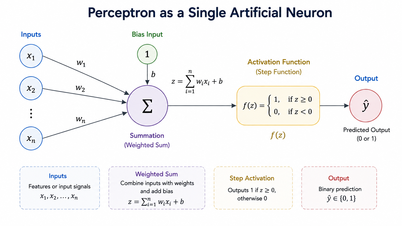
- perceptron প্রতিটি ইনপুটকে একটি weight (ওয়েট) দিয়ে গুণ করে, যা বলে দেয় যে ওই ইনপুটটি কতটা গুরুত্বপূর্ণ। এরপর সেগুলোকে সব একসাথে যোগ করে, এবং এর সাথে আরও একটি সংখ্যা যোগ করে যাকে বলা হয় bias (বায়াস), যা সিদ্ধান্তটিকে ডানে বা বামে সরায়।
- যদি সেই যোগফল একটি নির্দিষ্ট থ্রেশহোল্ড (threshold) অতিক্রম করে, তবে এটি "হ্যাঁ" (ক্লাস 1) হিসেবে ফায়ার করে। অন্যথায় এটি চুপ থাকে ("ক্লাস 0")।
জ্যামিতিকভাবে, "যোগফল একটি থ্রেশহোল্ড অতিক্রম করে" কথাটির মানে হলো "পয়েন্টটি রেখার একপাশে অবস্থিত।" দ্বিমাত্রিক বা 2D স্পেসে এই সীমানা বা বাউন্ডারিটি একটি সরলরেখা। ত্রিমাত্রিক বা 3D স্পেসে এটি একটি সমতল পৃষ্ঠ বা প্লেন (plane)। আরও উচ্চতর ডাইমেনশনে — বাস্তব দুনিয়ার বেশিরভাগ প্রবলেম যেখানে থাকে — একে বলা হয় hyperplane (হাইপারপ্লেন), তবে মূল ধারণা কখনোই বদলায় না: perceptron সবসময় ডেটার মাঝখান দিয়ে শুধু একটি সরল কাট বা রেখা শিখতে পারে।
Perceptron প্লেগ্রাউন্ড
দুটি ক্লাসের জন্য পয়েন্ট যোগ করুন, তারপর লার্নিং রুলটি ধাপে ধাপে চালান এবং দেখুন কীভাবে ভুলগুলো শুধরানোর জন্য বাউন্ডারি লাইনটি সরে যায়।
Click the grid to add a point:
w = (0.10, 0.10), b = 0.00
জ্যামিতিকভাবে ওয়েট ও বায়াসের ভূমিকা (What Weight and Bias Control, Geometrically)
সমীকরণে যাওয়ার আগে আরেকটু জ্যামিতিক অন্তর্দৃষ্টি তৈরি করে নেওয়া যাক, কারণ এটি সামনের প্রায় প্রতিটি চ্যাপ্টারে কাজে লাগবে। ওয়েট ভেক্টর আসলে ডিসিশন বাউন্ডারির (রেখা বা হাইপারপ্লেন) সাথে সবসময় লম্ব (perpendicular) থাকে — এটি নির্দেশ করে বাউন্ডারিটি ঠিক কোন দিকে মুখ করে আছে। -এর দিক বদলালে রেখাটি ঘুরে যায়; কিন্তু -এর ম্যাগনিচিউড বা মান বাড়ালে-কমালে রেখাটির অবস্থান একদমই বদলায় না, শুধু -এর মান কতটা দ্রুত বাড়ে বা কমে তা বদলায় (অর্থাৎ বাউন্ডারি থেকে দূরে সরে গেলে কনফিডেন্স কত দ্রুত বাড়ে)। অন্যদিকে, বায়াস পুরো রেখাটিকে মূলবিন্দুর (origin) দিকে বা তার থেকে দূরে ঠেলে দেয়, ওয়েটের দিক না বদলিয়েই। মনে রাখার একটি সহজ উপায়: ওয়েট ঠিক করে রেখাটি কোন দিকে হেলে থাকবে, বায়াস ঠিক করে রেখাটি কতদূর সরে যাবে।
এর পেছনের গণিত (The Math Behind It)
প্রেডিকশন বা ভবিষ্যদ্বাণী করা (Making a Prediction)
যেখানে: হলো ইনপুট ফিচার ভেক্টর, হলো ওয়েট ভেক্টর, হলো বায়াস, হলো প্রি-অ্যাক্টিভেশন (pre-activation বা raw ওয়েটেড সাম), হলো হেভিসাইড স্টেপ ফাংশন (Heaviside step function), এবং হলো প্রেডিক্ট করা ক্লাস লেবেল (0 বা 1)।
সহজ কথায়: সেট করলেই বাউন্ডারিটি সংজ্ঞায়িত হয়ে যায় — হলো সেই আলাদা করা হাইপারপ্লেনের সমীকরণ। এর একপাশের সবকিছুকে 1 এবং অন্য পাশের সবকিছুকে 0 হিসেবে প্রেডিক্ট করা হয়। ওয়েটগুলো ওই বাউন্ডারির ওরিয়েন্টেশন (orientation) বা দিক নিয়ন্ত্রণ করে; আর বায়াস নিয়ন্ত্রণ করে বাউন্ডারিটি মূলবিন্দু (origin) থেকে কতটা দূরে থাকবে।
ভুল থেকে শেখা (Learning From Mistakes)
আসল চালাকিটা নিউরনে ছিল না — একই ধরনের মডেল কয়েক বছর আগেই অস্তিত্বে ছিল। Rosenblatt-এর আসল অবদান ছিল ভালো ওয়েটগুলো স্বয়ংক্রিয়ভাবে খুঁজে বের করার একটি অত্যন্ত সহজ, এবং নিশ্চিত নিয়ম।
যেখানে: হলো লার্নিং রেট বা learning rate (প্রতিটি সংশোধনের পরিমাণ কতটা বড় হবে), হলো আসল বা ট্রু লেবেল, হলো প্রেডিক্ট করা লেবেল, এবং হলো প্রেডিকশনের এরর (error) বা ভুল।
সহজ কথায়: যদি প্রেডিকশন আগে থেকেই ঠিক থাকে, তবে হয় এবং কোনো কিছুই বদলায় না — perceptron কখনোই এমন কোনো ওয়েটকে ছোঁয় না যা ছোঁয়ার দরকার নেই। যদি সে 0 প্রেডিক্ট করে কিন্তু আসল উত্তর 1 হয়, তবে এরর হলো , এবং প্রতিটি ওয়েটকে ওই ইনপুটের দিকে একটু ধাক্কা দেওয়া হয়, যাতে পরের বার আরেকটু বড় হয়। যদি ঠিক উল্টোটা হয়, তবে ধাক্কাটা উল্টো দিকে লাগে। এটি হলো সবচেয়ে ছোট সম্ভাব্য সংশোধন যা ঠিক তার সামনের ভুলটাকে শুধরে দেয়।
এটি gradient descent-এর একটি স্পেশাল কেস
Perceptron রুলটিকে দেখতে হাতে বানানো মনে হলেও, এটি আসলে এমন একটি লস ফাংশনের (যাকে "perceptron criterion" বলা হয়) ওপর চালানো gradient descent, যা কেবল ভুলভাবে ক্লাসিফাই করা পয়েন্টগুলোকেই পেনাল্টি দেয়। অপ্টিমাইজেশন থিওরি (optimization theory) বলতে কী বোঝায় তা চ্যাপ্টার ১২-তে বিস্তারিত দেওয়া আছে; perceptron শব্দটি জনপ্রিয় হওয়ার কয়েক দশক আগেই এটি এই কাজটি করে আসছিল।
কনভার্জেন্স গ্যারান্টি — এবং এর শর্ত (The Convergence Guarantee — and Its Catch)
যদি ট্রেনিং ডেটা linearly separable হয় (অর্থাৎ একটি সরলরেখা দিয়ে আলাদা করা যায়), তবে perceptron লার্নিং অ্যালগরিদমটি নির্দিষ্ট সংখ্যক ধাপের মধ্যেই এমন সব ওয়েট খুঁজে পেতে নিশ্চিতভাবে কনভার্জ (converge) করবে, যা প্রতিটি ট্রেনিং উদাহরণকে নিখুঁতভাবে ক্লাসিফাই করতে পারে।
গ্যারান্টির একটি কঠিন পূর্বশর্ত আছে
উপরের থিওরেমে "Linearly separable" কথাটিই আসল কাজ করছে। যদি কোনো সরলরেখা দিয়ে দুটি ক্লাসকে আলাদা করা সম্ভব না হয়, তবে perceptron কখনোই শান্ত হবে না — এটি অনন্তকাল ধরে দুলতে (oscillate) থাকবে, একটি পয়েন্ট ঠিক করতে গিয়ে অন্য আরেকটি পয়েন্ট ভুল করে ফেলবে। ঠিক এই একটি সীমাবদ্ধতাই হলো পরের চ্যাপ্টারের মূল বিষয়, আর এটিই প্রথম AI winter-এর সূচনা করেছিল।
তাহলে non-separable ডেটার ক্ষেত্রে কী করা হয়?
এই সীমাবদ্ধতা মোকাবিলা করার জন্য পরবর্তীতে একটি ছোট পরিবর্তন প্রস্তাব করা হয়েছিল, যাকে বলা হয় pocket algorithm: ট্রেনিংয়ের সময় এখন পর্যন্ত পাওয়া সবচেয়ে ভালো ওয়েট সেটটি (যেটি সবচেয়ে কম ভুল করে) আলাদাভাবে "পকেটে" জমা রাখা হয়, এবং লুপ শেষে ওই সেরা ওয়েটটিই আউটপুট দেওয়া হয় — এটি কনভার্জেন্স গ্যারান্টি করে না, কিন্তু অন্তত একটি ব্যবহারযোগ্য আনুমানিক সমাধান দেয়। তবে সত্যিকারের সমাধান, যা এই সীমাবদ্ধতাকে পুরোপুরি ভিন্নভাবে মোকাবিলা করে, তা আসে পরের দুটি চ্যাপ্টার থেকে।
হাতে-কলমে উদাহরণ: লজিক্যাল AND শেখা (Worked Example: Learning Logical AND)
চলুন একটি perceptron কীভাবে AND ফাংশন শেখে তা হাতে-কলমে মিলিয়ে দেখি। ধরে নিই শুরুতে সব ওয়েট জিরো (zero) এবং লার্নিং রেট ।
| x₁ | x₂ | y (AND) |
|---|---|---|
| 0 | 0 | 0 |
| 0 | 1 | 0 |
| 1 | 0 | 0 |
| 1 | 1 | 1 |
Epoch 1, উদাহরণ (0, 0), : (ভুল)। Error , তাই (ওয়েটগুলো 0-ই থাকবে, কারণ )।
Epoch 1, উদাহরণ (0, 1), : — সঠিক, কোনো আপডেট নেই।
Epoch 1, উদাহরণ (1, 0), : — সঠিক, কোনো আপডেট নেই।
Epoch 1, উদাহরণ (1, 1), : (ভুল)। Error , তাই , , ।
এক ইপোক (epoch) পর: । এই একই চেক-অ্যান্ড-কারেক্ট (check-and-correct) লুপটি আরও কয়েক ইপোক চালালে তা এমন কিছুতে কনভার্জ করে যেমন , যার ফলে পাওয়া যায় — যা ৪টি সারির জন্য ঠিক তৈরি করে, এবং প্রেডিকশন দেয় । এটিই হলো AND ট্রুথ টেবিল (truth table), যা পুরোপুরি ভুল থেকে শেখা হয়েছে।
পরীক্ষার কৌশল (Exam technique)
হাতে-কলমে perceptron আপডেট ট্রেস করার সময়, একটি টেবিল তৈরি করে নিন যেখানে এর কলাম থাকবে। এটি যোগ-বিয়োগের ভুল এড়াতে সাহায্য করে এবং আংশিক নাম্বার দেওয়ার ক্ষেত্রে পরীক্ষকের জন্য কাজটা সহজ করে।
OR গেট: আরেকটি দ্রুত উদাহরণ (OR Gate: A Quick Second Example)
AND-এর মতো একই লজিকে OR ফাংশনও শেখা যায়, শুধু ট্রুথ টেবিলটা বদলে যায়। AND-এর ক্ষেত্রে perceptron শুধু -এর বেলাতেই "হ্যাঁ" বলতে শেখে, কিন্তু OR-এর ক্ষেত্রে তিনটি ইনপুট কম্বিনেশনেই — , এবং — "হ্যাঁ" বলতে হয়, শুধু বাদে। একই check-and-correct লুপ চালালে তা কনভার্জ করে এমন একটি সমাধানে, যেমন — যা দেয় , ফলে -এর জন্য (না) আর বাকি তিনটির জন্য (হ্যাঁ)। লক্ষ করুন, শুধু বায়াসের মানটাই বদলে গেছে ( থেকে -এ) — এটিই দেখায় কীভাবে বায়াস একা বাউন্ডারিকে সরিয়ে সম্পূর্ণ ভিন্ন একটি লজিক্যাল ফাংশন তৈরি করে দিতে পারে, ওয়েটের দিক না বদলিয়েই।
Implementation
python
এই কোডটি সম্পর্কে কিছু জিনিস খেয়াল করার মতো:
- এখানে জিরো দিয়ে ইনিশিয়ালাইজ (Zero-initialized) করা ওয়েট ঠিক আছে। একটি মাত্র perceptron-এর ক্ষেত্রে সিমেট্রি প্রবলেম (symmetry problem) নেই — প্রতিটি ওয়েট একদম একই দিয়ে শুরু হলেও, যেহেতু এখানে একটাই নিউরন, তাই ব্রেক করার মতো নিউরনগুলোর মাঝে কোনো সিমেট্রি নেই। যখন আমরা লেয়ারের পর লেয়ার স্ট্যাক করব (চ্যাপ্টার ১৮), তখন এটি বদলে যাবে।
- ট্রেনিং লুপটি আগেভাগেই থেমে যায় যখন একটি সম্পূর্ণ ইপোক-এ ভুলের পরিমাণ জিরো হয় — কনভার্জেন্স থিওরেম গ্যারান্টি দেয় যে, ডেটা linearly separable হলে শেষ পর্যন্ত এমনটা ঘটবেই।
predict-ই হলো পুরো ফরোয়ার্ড পাস (forward pass)। এখানে কোনো হিডেন লেয়ার নেই, একগাদা ম্যাট্রিক্স মাল্টিপ্লিকেশনের কোনো চেইন নেই — শুধু একটি ডট প্রোডাক্ট (dot product) আর জিরোর সাথে একটি তুলনা।
মূল বিষয়গুলো (Key Takeaways)
Key Takeaways
- perceptron হলো একটি লিনিয়ার বাইনারি ক্লাসিফায়ার: , যেখানে স্টেপ অ্যাক্টিভেশন ব্যবহার করা হয়।
- এর ডিসিশন বাউন্ডারি (decision boundary) হলো একটি হাইপারপ্লেন, যাকে দিয়ে সংজ্ঞায়িত করা হয়।
- লার্নিং রুলটি শুধু সেই উদাহরণগুলোর ওয়েট আপডেট করে যেগুলো ভুলভাবে ক্লাসিফাই হয়েছে: ।
- Perceptron Convergence Theorem কনভার্জেন্সের গ্যারান্টি দেয় — তবে শুধুমাত্র linearly separable ডেটার জন্য।
- এটি AND, OR, এবং একই ধরনের ফাংশনগুলো শিখতে পারে, কিন্তু পরের চ্যাপ্টারে যেমনটা দেখানো হবে, এটি কোনোভাবেই XOR শিখতে পারে না।
সাধারণ ভুল ধারণা (Common Mistakes)
বায়াস (bias) টার্ম ভুলে যাওয়া
বায়াস ছাড়া ডিসিশন বাউন্ডারিকে মূলবিন্দু (origin) দিয়ে যেতে বাধ্য করা হয়। এটি একটি বিশাল ও অপ্রয়োজনীয় সীমাবদ্ধতা — সবসময় অন্য যেকোনো ওয়েটের মতোই বায়াস যুক্ত করুন এবং তাকে ট্রেন করুন।
ধরে নেওয়া যে perceptron সবসময়ই কনভার্জ করবে
কনভার্জেন্স থিওরেমের একটি পূর্বশর্ত রয়েছে যা তাড়াহুড়োয় এড়িয়ে যাওয়া খুব সহজ: ডেটাকে linearly separable হতে হবে। বাস্তব দুনিয়ার অনেক ডেটাসেটই এমন হয় না, আর সেসব ক্ষেত্রে ট্রেনিং লস জিরো হওয়ার বদলে অনন্তকাল ধরে দুলতে (oscillate) থাকবে।
ওয়েটের ম্যাগনিচিউড আর কনফিডেন্সকে গুলিয়ে ফেলা
স্টেপ অ্যাক্টিভেশনে -এর প্রকৃত মান কোনো ভূমিকা রাখে না — শুধু এর সাইন (sign) গুরুত্বপূর্ণ। তাই এবং উভয়ই একই প্রেডিকশন দেয়, যদিও দ্বিতীয়টি বাউন্ডারি থেকে অনেক দূরে। perceptron নিজে থেকে কোনো "কনফিডেন্স স্কোর" দেয় না — সেই ক্ষমতা আসে পরের চ্যাপ্টারে যখন sigmoid-এর মতো মসৃণ অ্যাক্টিভেশন ফাংশন ব্যবহার করা শুরু হয়।
ইন্টারভিউ কর্নার (Interview Corner)
Quick Check
বাস্তবে এটি কোথায় দেখা যায় (Where This Shows Up in Practice)
আজকাল একা একা বা স্ট্যান্ড-অ্যালোন (standalone) perceptron-এর ব্যবহার খুব একটা দেখা যায় না, কিন্তু ধারণাটি কখনোই হারিয়ে যায়নি — এটি আধুনিক Neural Network-এর প্রতিটি নিউরনের বেসিক বিল্ডিং ব্লকে পরিণত হয়েছে। একটি মাত্র perceptron ঠিক কী করতে পারে আর কী পারে না তা বুঝতে পারাই হলো ডিপ লার্নিং কেন এতগুলো perceptron-কে একসাথে সাজায় তা বোঝার সবচেয়ে দ্রুত পথ, আর ঠিক সেই জায়গাতেই পরের দুটি চ্যাপ্টার এগিয়ে যাচ্ছে।