Chapter 21 of 25
Practical Implementation
Building an MLP for real, bugs and all
17 min read
Created ২ আগ, ২০২৬
ভূমিকা (Motivation)
ফরওয়ার্ড পাস, ব্যাকপ্রোপাগেশন এবং ট্রেনিং লুপের ব্যাপারে পড়া এক জিনিস, আর বাস্তবে একটি এডিটর খুলে, কোনো লাইব্রেরি ইম্পোর্ট করে আসল ডেটার ওপর একটি নেটওয়ার্ক ট্রেন করা সম্পূর্ণ ভিন্ন একটি দক্ষতা — এবং এটিই কোনো একটি কনসেপ্ট বা ধারণা কেবল মুখে বোঝার থেকে সেটিকে বাস্তবে ব্যবহার করতে পারার মধ্যে পার্থক্য গড়ে দেয়। ভালো খবর হলো, এতক্ষণ পর্যন্ত আমরা তাত্ত্বিকভাবে যা কিছু শিখেছি তার প্রতিটি অংশ যেকোনো আধুনিক ফ্রেমওয়ার্কে মাত্র কয়েক লাইনের কোডের সাথে সরাসরি মিলে যায়। আর খারাপ খবর হলো, প্রতিটি ফ্রেমওয়ার্ক ঠিক এই একই ধারণাগুলোকে আলাদা আলাদা ডিফল্ট মান, আলাদা লেভেলের সুযোগ-সুবিধা এবং খুব সূক্ষ্মভাবে কোনো ভুল করে ফেলার মতো আলাদা আলাদা ফাঁদ দিয়ে প্রকাশ করে।
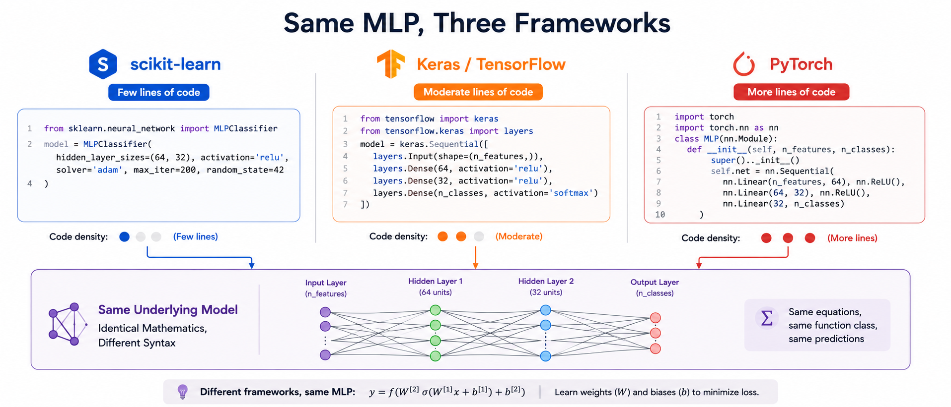
এই চ্যাপ্টারটি ঠিক এই অমিলটুকুই দূর করবে। আমরা একই কাজকে তিনটি ভিন্ন ভিন্ন ফ্রেমওয়ার্ক — scikit-learn, TensorFlow/Keras, এবং PyTorch — দিয়ে তিনবার ইমপ্লিমেন্ট করব, যাতে আপনি পাশাপাশি রেখে দেখতে পারেন যে পেছনের গণিত এক হওয়া সত্ত্বেও এদের ভেতরের অ্যাবস্ট্রাকশনগুলো (abstractions) কীভাবে আলাদা কাজ করে।
একটি বাস্তব জীবনের উদাহরণ (A Real-Life Scenario)
ভাবুন তো, একটি হাসপাতালের ডেটা সায়েন্স টিম কোষ বা সেলের পরিমাপ করা বিভিন্ন ফিচার থেকে একটি টিউমার ম্যালিগন্যান্ট বা ক্ষতিকারক হওয়ার সম্ভাবনা আছে কি না তা ফ্ল্যাগ করার জন্য একটি মডেল তৈরি করছে — এটি টেবুলার ডেটার ওপর একটি বাস্তব এবং খুব গুরুত্বপূর্ণ বাইনারি ক্লাসিফিকেশন (binary classification) समस्या, যা বহুল পরিচিত Breast Cancer Wisconsin ডেটাসেটের ধারণার কাছাকাছি। টিমের একজন জুনিয়র মেম্বার হয়তো scikit-learn ব্যবহার করে মাত্র ১০ লাইনেই একটি সাধারণ বেসলাইন (baseline) তৈরি করে ফেলতে পারেন। টিমের অন্য কেউ যে জিপিইউ ক্লাস্টারে বড় পরিসরে মডেলটি ডেপ্লয় বা স্থাপন করার প্রস্তুতি নিচ্ছেন, তিনি হয়তো Keras ব্যবহার করতে চাইবেন। আবার অন্য একটি রিসার্চ বা গবেষণা টিম যারা একটি সম্পূর্ণ কাস্টম বা অদ্ভুত কোনো আর্কিটেকচার নিয়ে পরীক্ষা করতে চাইছে, তাদের জন্য হয়তো PyTorch-এর সম্পূর্ণ ফ্লেক্সিবিলিটি বা স্বাধীনতার প্রয়োজন হবে। তারা তিনজনই কিন্তু একই সমস্যার সমাধান করছেন — ফ্রেমওয়ার্ক বেছে নেওয়াটা একটি ব্যবহারিক ইঞ্জিনিয়ারিং সিদ্ধান্ত, গাণিতিক কোনো বিষয় নয়।
কাজের প্রস্তুতি (Task Setup)
আমরা টেবুলার ডেটার ওপর একটি বাইনারি ক্লাসিফিকেশন কাজ ব্যবহার করব — ফিচার পরিমাপ করে একটি টিউমার ম্যালিগন্যান্ট বা ক্ষতিকারক কি না তা প্রেডিক্ট করব — Predicting whether a tumor is malignant from measured numeric features — যেখানে ট্রেনিং পাইপলাইন চ্যাপ্টারের পরামর্শ অনুযায়ী সব ইনপুট ফিচারকে জিরো মিন (zero mean) এবং ইউনিট ভ্যারিয়েন্সে (unit variance) স্ট্যান্ডার্ডাইজ করা হয়েছে।
কেন একই সমস্যা তিনবার সমাধান করছি (Why Solve the Same Problem Three Times)
এই পুনরাবৃত্তিটি ইচ্ছাকৃত। যখন আপনি একটি নতুন ফ্রেমওয়ার্ক শিখছেন, তখন সবচেয়ে বড় ঝুঁকিটি হলো এই বিভ্রান্তি যে "নতুন সিনট্যাক্স" আর "নতুন গণিত" — এই দুটো আসলে একই জিনিস। বাস্তবে তা নয়। তিনটি ইমপ্লিমেন্টেশনই ঠিক একই ফরওয়ার্ড পাস, একই লস ফাংশনের ধারণা এবং একই গ্রেডিয়েন্ট-ভিত্তিক অপ্টিমাইজেশন প্রয়োগ করছে — শুধু এদের API-র "চেহারা" আলাদা। একবার এই তিনটি কোড পাশাপাশি রেখে দেখলে, ভবিষ্যতে চতুর্থ কোনো ফ্রেমওয়ার্ক (যেমন JAX বা কোনো নতুন লাইব্রেরি) শেখার সময়ও আপনি জানবেন ঠিক কোন কোন প্রশ্ন করতে হবে: ওয়েট কীভাবে ইনিশিয়ালাইজ হয়, ট্রেনিং ও ইভাল মোড কীভাবে সুইচ হয়, এবং গ্রেডিয়েন্ট কীভাবে হিসাব ও প্রয়োগ করা হয়।
কীভাবে এই চ্যাপ্টার পড়বেন (How to read this chapter)
প্রতিটি ইমপ্লিমেন্টেশন একবার নিজে হাতে চালিয়ে দেখুন, তারপর তিনটি কোড একে অপরের পাশে রেখে মিলিয়ে দেখুন কোন লাইনটি কোন লাইনের সমতুল্য। এই "সাইড-বাই-সাইড" পড়ার পদ্ধতিটিই একটি নতুন ফ্রেমওয়ার্ক শেখার দ্রুততম পথ, কারণ আপনি সবসময় জানবেন গণিতের কোন অংশটি এখন কোন সিনট্যাক্সে লুকিয়ে আছে।
ইমপ্লিমেন্টেশন ১: scikit-learn
python
খেয়াল করুন এখানে কত কিছু আড়ালে বা ইমপ্লিসিটলি (implicitly) ঘটে গেছে: hidden_layer_sizes=(64, 32) অংশটি নিজে হাতে কোনো ম্যাট্রিক্স শেপ বা আকার না লিখেই পুরো আর্কিটেকচারটি ডিফাইন করে ফেলেছে, alpha হলো আমরা আগে আলোচনা করা L2 রেগুলারাইজেশনের শক্তি বা স্ট্রেন্থ, এবং validation_fraction=0.15 এর সাথে early_stopping=True খুব নীরবে একটি ভ্যালিডেশন স্প্লিট তৈরি করে আপনার জন্য সেটির পারফরম্যান্স ট্র্যাক করেছে। এখানে কোডে সরাসরি কোনো ট্রেনিং লুপ দেখাই যাচ্ছে না — .fit() কলটি আগের চ্যাপ্টারের পুরো পাইপলাইনটি নিজের ভেতরেই স্বয়ংক্রিয়ভাবে রান করিয়ে নেয়।
ব্যবহারিক নোট: টেবুলার ডেটা এবং খুব দ্রুত কোনো বেসলাইন তৈরির জন্য scikit-learn-এর MLPClassifier হলো সবচেয়ে কম কোড লিখে একটি কার্যকরী MLP পাওয়ার সবচেয়ে সহজ উপায়। এটি ট্রেনিং লুপকে পুরোপুরি লুকিয়ে ফেলে এবং Keras বা PyTorch-এর তুলনায় কম ফ্লেক্সিবিলিটি বা সুযোগ দেয় — এতে কোনো কাস্টম আর্কিটেকচার তৈরি করা যায় না, এবং সবচেয়ে বড় কথা হলো, এতে কোনো জিপিইউ (GPU) সাপোর্ট নেই।
scikit-learn-এ কাজ করার সময়কার ডিবাগিং টিপস (Debugging Tips for scikit-learn)
যেহেতু MLPClassifier-এর ট্রেনিং লুপটি সম্পূর্ণভাবে লুকানো থাকে, তাই এখানে ভুল হলে তা ধরা একটু কঠিন হতে পারে। কিছু ব্যবহারিক পরামর্শ:
model.loss_curve_প্লট করুন। ফিট করার পর এই অ্যাট্রিবিউটে প্রতিটি ইপোকের ট্রেনিং লস জমা থাকে। যদি এই কার্ভটি সমতল বা একদম শুরুতেই আটকে যায়, তাহলে লার্নিং রেট খুব ছোট, অথবা ফিচারগুলো ঠিকভাবে স্ট্যান্ডার্ডাইজ করা হয়নি।ConvergenceWarning-কে উপেক্ষা করবেন না। এই ওয়ার্নিংটি বলে দেয় যেmax_iter-এর মধ্যে অপ্টিমাইজার কনভার্জ করতে পারেনি। প্রথম সমাধান হলোmax_iterবাড়ানো, কিন্তু যদি বহুগুণ বাড়ানোর পরও কাজ না হয়, তাহলে লার্নিং রেট বা ইনপুট স্কেলিং নিয়ে সন্দেহ করুন।n_iter_no_changeএবংtolপ্যারামিটার দুটো একসাথে কাজ করে early stopping কতটা "ধৈর্যশীল" হবে তা নিয়ন্ত্রণ করতে — এগুলো ঠিক Keras/PyTorch-এর patience-এর মতোই আচরণ করে, শুধু নাম আলাদা।
ইমপ্লিমেন্টেশন ২: TensorFlow / Keras
python
এখানের প্রতিটি লাইনের সাথেই আমাদের আগের চ্যাপ্টারগুলোর সরাসরি সংযোগ আছে: kernel_initializer="he_normal" হলো ReLU-এর সাথে ব্যবহার করা He ইনিশিয়ালাইজেশন স্কিম, BatchNormalization() and Dropout(0.3) হলো আগে আলোচনা করা রেগুলারাইজেশন টেকনিকগুলো, এবং restore_best_weights=True এর সাথে EarlyStopping কলব্যাকটি ঠিক আগের চ্যাপ্টারের বলা সবচেয়ে সেরা চেকপয়েন্টটি ফিরিয়ে আনার পরামর্শ অনুযায়ী কাজ করে। প্রথম Dense লেয়ারের use_bias=False অংশটি খেয়াল করুন — ব্যাচ নরমালাইজেশন (Batch Normalization) যখন নিজের লার্নেবল শিফট দিয়ে দেয়, তখন এই বায়াসটি আসলেই অপ্রয়োজনীয় বা redundant হয়ে যায়।
ব্যবহারিক নোট: Keras-এর Sequential/Functional API এই কোর্সের লেয়ার-বাই-লেয়ার নোটেশনের বা ব্যাখ্যার সাথে একদম সরাসরি মিলে যায়: প্রতিটি Dense লেয়ার একটি ওয়েট-অ্যান্ড-বায়াস জুটির সাথে মিলে যায়। Keras অটোমেটিক ডিফারেনসিয়েশনের (automatic differentiation) মাধ্যমে ব্যাকপ্রোপাগেশন নিজেই সামলে নেয় — আপনাকে নিজে হাতে কোনো গ্রেডিয়েন্ট ফর্মুলা লিখতে হয় না।
Keras-এ কাজ করার সময়কার সাধারণ সমস্যাগুলো (Common Gotchas in Keras)
Keras-এর ডিক্লেয়ারেটিভ (declarative) স্টাইলটি অনেক কিছু সহজ করে দেয়, কিন্তু ঠিক এই সহজতার কারণেই কিছু ভুল একদম নীরবে ঘটে যায় এবং প্রথম দেখায় বোঝা কঠিন হয়:
model.summary()কল করুন প্রথমেই। ফিট করার আগে এটি প্রতিটি লেয়ারের আউটপুট শেপ এবং প্যারামিটার সংখ্যা দেখিয়ে দেয় — যদি কোনো শেপ প্রত্যাশার চেয়ে আলাদা দেখায়, তাহলে ট্রেনিং শুরু হওয়ার আগেই সমস্যাটি ধরা পড়ে যাবে।- লস হঠাৎ
NaNহয়ে গেলে, প্রথমে লার্নিং রেট কমান, এরপর চেক করুন ইনপুটে কোনোinfবাNaNমান আছে কি না।BatchNormalizationএবং খুব উঁচু লার্নিং রেট একসাথে থাকলে এটি প্রায়ই ঘটে। history.historyডিকশনারিটি ট্রেনিং এবং ভ্যালিডেশন উভয় লস/মেট্রিক সংরক্ষণ করে — ট্রেনিং লস কমছে অথচ ভ্যালিডেশন লস বাড়ছে দেখলে সেটিই ওভারফিটিং-এর সবচেয়ে স্পষ্ট সংকেত, এবং তখনই রেগুলারাইজেশন বাড়ানো বা early stopping-এর patience কমানো দরকার।
ইমপ্লিমেন্টেশন ৩: PyTorch
python
এই কোড সংস্করণটি বা ভার্সনটি নিজে হাতে প্রতিটি কাজ লিখে দেখায় যা Keras আড়ালে করছিল। for epoch in range(100) লুপটি হলো আগের চ্যাপ্টারে আলোচনা করা ট্রেনিং-লুপ অ্যালগরিদমের একদম হুবহু ও সরাসরি ইমপ্লিমেন্টেশন। model.train() এবং model.eval() হলো সেই সুনির্দিষ্ট বা এক্সপ্লিসিট মোড সুইচ, যার ওপর ড্রপআউট এবং ব্যাচ নরমালাইজেশন উভয়েই নির্ভর করে — যেকোনো একটি বাদ দিলেই ট্রেনিং এবং ইনফারেন্সের আচরণ নীরবে ভুল পথে চলে যাবে। loss.backward() কলটি নিজে হাতে কোনো গ্রেডিয়েন্ট ফর্মুলা লেখা ছাড়াই অটোমেটিক ডিফারেনসিয়েশনের মাধ্যমে আগে আলোচনা করা ব্যাকপ্রোপাগেশন অ্যালগরিদমটি হুবহু সম্পন্ন করে। ভ্যালিডেশন পারফরম্যান্স ভালো হওয়ার পর প্রতিবার best_state সেভ করে রাখার ম্যানুয়াল বা নিজে হাতে লেখা patience_ctr ব্লকটি মূলত কোনো কলব্যাকের পেছনে না লুকিয়ে থেকে নিজে হাতে স্ক্র্যাচ থেকে আর্লি স্টপিং ইমপ্লিমেন্ট করার চমৎকার উদাহরণ।
কেন sigmoid + BCELoss-এর বদলে BCEWithLogitsLoss ব্যবহার করা হয়
BCEWithLogitsLoss সিগময়েড অ্যাক্টিভেশন এবং বাইনারি ক্রস-এন্ট্রপি লসকে একটিমাত্র গাণিতিকভাবে স্থিতিশীল operasione যুক্ত করে, যা আলাদা করে প্রোবাবিলিটি বা সম্ভাবনা ক্যালকুলেট করার বদলে সরাসরি raw লজিট (logit)-এর ওপর হিসাব করা হয়। ঠিক এই কারণেই ওপরে নেটওয়ার্কের শেষ Linear লেয়ারটিতে কোনো অ্যাক্টিভেশন দেওয়া হয়নি — লস ফাংশনটি নিজের ভেতরেই সিগময়েড অ্যানালিসিস করে নেয়, যা -এর মান অনেক বড় পজিটিভ বা নেগেটিভ হলে আলাদা আলাদা ফ্লোটিং-পয়েন্ট ধাপে ক্যালকুলেট করার গাণিতিক অস্থিতিশীলতা পুরোপুরি দূর করে। এটি ব্যাকপ্রোপাগেশন প্রথম আবিষ্কারের সময় প্রমাণ করা গ্রেডিয়েন্টের সেই সরল রূপটিই কাজে লাগায়।
ব্যবহারিক নোট: PyTorch-এর ক্ষেত্রে ট্রেনিং লুপটি কোডে নিজে হাতে লিখতে হয়, যার ফলে ট্রেনিং পাইপলাইনের প্রতিটি ধাপ সরাসরি কোডের চোখে ভেসে ওঠে। এটি একটু বেশি বড় বা ভারবোস (verbose) মনে হলেও ঠিক এই কারণেই রিসার্চ বা কাস্টম আর্কিটেকচার তৈরির জন্য PyTorch-কে বেশি পছন্দ করা হয় — স্ট্যান্ডার্ড বা সাধারণ API যা আশা করে না এমন কিছু করার সময় এখানে কোনো লুকানো আচরণ নিয়ে ঝামেলা পোহাতে হয় না।
PyTorch-এ সবচেয়ে বেশি হওয়া ভুলগুলো (The Most Common PyTorch Mistakes)
PyTorch যেহেতু ট্রেনিং লুপের প্রতিটি ধাপ নিজে হাতে লিখতে বাধ্য করে, তাই এখানে ভুল হওয়ার সুযোগও বেশি — কিন্তু ঠিক এই কারণেই ভুলগুলো খুঁজে বের করাও তুলনামূলক সহজ, কারণ প্রতিটি ধাপ চোখের সামনে থাকে।
optimizer.zero_grad() ভুলে যাওয়া
PyTorch ডিফল্টভাবে গ্রেডিয়েন্ট জমা করতে থাকে (accumulate করে)। প্রতিটি নতুন ব্যাচের আগে zero_grad() কল না করলে গ্রেডিয়েন্টগুলো একের পর এক যোগ হতে থাকে এবং ট্রেনিং সম্পূর্ণ ভুল পথে চলে যায়।
টেন্সর ও মডেল ভিন্ন ডিভাইসে থাকা
মডেল GPU-তে (.to("cuda")) কিন্তু ইনপুট টেন্সর এখনও CPU-তে থাকলে RuntimeError আসে। মডেল এবং ডেটা — দুটোকেই একই ডিভাইসে পাঠাতে হবে।
শেপ মিসম্যাচ নীরবে ব্রডকাস্ট হয়ে যাওয়া
y_train-কে unsqueeze(1) না করলে prediction shape (N, 1) এবং টার্গেট shape (N,) ব্রডকাস্টিং-এর মাধ্যমে ভুলভাবে মিলে যায় এবং লস চুপচাপ ভুল মান দেয় — কোনো এরর ছাড়াই।
with torch.no_grad() ছাড়া ইনফারেন্স করা
ভ্যালিডেশন বা টেস্টের সময় গ্রেডিয়েন্ট ট্র্যাক করার দরকার নেই। no_grad() ব্লক না ব্যবহার করলে অহেতুক মেমরি খরচ হয় এবং বড় মডেলে সহজেই আউট-অফ-মেমরি এরর দেখা দিতে পারে।
একটি সাধারণ ডিবাগিং অভ্যাস হলো ট্রেনিং শুরু করার আগে ইচ্ছা করে একটি ছোট সাবসেট (যেমন মাত্র ৮-১৬টি স্যাম্পল) দিয়ে মডেলটিকে বহু ইপোক ধরে ওভারফিট করানোর চেষ্টা করা:
python
যদি একটি ১৬-স্যাম্পলের ব্যাচেই লস প্রায় শূন্যে নামতে না পারে, তাহলে সমস্যাটি হাইপারপ্যারামিটার টিউনিং-এর নয় — বরং কোডে কোথাও একটি বাগ (bug) লুকিয়ে আছে, যেমন ভুল লস ফাংশন, ভুল শেপ, অথবা গ্রেডিয়েন্ট আসলে ফ্লো-ই করছে না।
ফ্রেমওয়ার্কের তুলনা (Framework Comparison)
| দিক বা Aspect | scikit-learn | Keras/TensorFlow | PyTorch |
|---|---|---|---|
| সহজ ব্যবহার | সবচেয়ে বেশি (মাত্র কয়েক লাইন) | অনেক ভালো (ডিক্লেয়ারেটিভ লেয়ার) | মাঝারি (নিজে হাতে লেখা লুপ) |
| ফ্লেক্সিবিলিটি বা স্বাধীনতা | কম (ফিক্সড MLP আর্কিটেকচার) | ভালো | সবচেয়ে বেশি |
| জিপিইউ (GPU) সাপোর্ট | নেই | আছে | আছে |
| যাদের জন্য ভালো | দ্রুত বেসলাইন তৈরি, টেবুলার ডেটা, শেখার কাজে | প্রোডাকশন ডেপ্লয়মেন্ট, প্রোটোটাইপ তৈরি | রিসার্চ, কাস্টম আর্কিটেকচার, পুঙ্খানুপুঙ্খ নিয়ন্ত্রণ |
বাস্তবে ফ্রেমওয়ার্ক বেছে নেওয়া (Choosing a framework in practice)
শেখার উদ্দেশ্যে, NumPy ব্যবহার করে একদম স্ক্র্যাচ থেকে একটি MLP-র ফরওয়ার্ড এবং backward পাস নিজে হাতে ইমপ্লিমেন্ট করাটাই হলো সবচেয়ে ভালো উপায় বোঝার জন্য যে এই ফ্রেমওয়ার্কগুলো আসলে এদের পেছনের API-র আড়ালে কী কী কাজ স্বয়ংক্রিয়ভাবে করে যাচ্ছে। বাস্তব প্রজেক্টের ক্ষেত্রে: খুব দ্রুত টেবুলার বেসলাইন তৈরি করতে scikit-learn ব্যবহার করুন, আর জিপিইউ, কাস্টম আর্কিটেকচার বা প্রোডাকশনে কাজের জন্য Keras অথবা PyTorch বেছে নিন।
প্রোডাকশনের জন্য মডেল সেভ ও লোড করা (Saving and Loading Models for Production)
ট্রেনিং শেষ হওয়ার পরও কাজ শেষ হয় না — বাস্তব প্রজেক্টে মডেলটিকে ডিস্কে সংরক্ষণ করে পরে আবার লোড করে ব্যবহার করতে হয়। তিনটি ফ্রেমওয়ার্কেই এই কাজটি একটু ভিন্নভাবে করা হয়:
python
স্কেলার সংরক্ষণ করতে ভুলে যাওয়া
মডেলের সাথে সাথে StandardScaler-টিকেও সংরক্ষণ করে রাখা আবশ্যক (যেমন joblib.dump(scaler, "scaler.joblib"))। প্রোডাকশনে নতুন ডেটা আসলে সেটিকে ঠিক একই মিন এবং স্ট্যান্ডার্ড ডিভিয়েশন দিয়ে ট্রান্সফর্ম করতে হবে যা ট্রেনিং সময়ে ব্যবহার করা হয়েছিল — নাহলে মডেলটি এমন ইনপুট দেখবে যা তার প্রশিক্ষণকালীন ডেটার সাথে সামঞ্জস্যপূর্ণ নয়, এবং প্রেডিকশন নীরবে ভুল হয়ে যাবে।
মূল বিষয়গুলো (Key Takeaways)
Key Takeaways
- scikit-learn-এর
MLPClassifierকম ফ্লেক্সিবিলিটি এবং জিপিইউ সাপোর্টের বিনিময়ে খুব কম কোড লিখে দ্রুততম সময়ে একটি ওয়ার্কিং বেসলাইন তৈরি করার সুযোগ দেয়। - Keras আর্কিটেকচারকে ডিক্লেয়ারেটিভ পদ্ধতিতে বা বর্ণনামূলকভাবে প্রকাশ করে, যা এই কোর্সের লেয়ার-বাই-লেয়ার ওয়েট-অ্যান্ড-বায়াস নোটেশনের সাথে চমৎকারভাবে মিলে যায়।
- PyTorch-এ একটি সুনির্দিষ্ট বা এক্সপ্লিসিট ট্রেনিং লুপ লিখতে হয়, যার ফলে প্রতিটি কনসেপ্ট — ফরওয়ার্ড পাস, লস, ব্যাকওয়ার্ড পাস, অপ্টিমাইজার ধাপ, আর্লি স্টপিং — সরাসরি কোডে দৃশ্যমান এবং পরিবর্তনযোগ্য থাকে।
- তিনটি ফ্রেমওয়ার্কই পেছনের হুবহু একই গণিত ইমপ্লিমেন্ট করে: ফরওয়ার্ড প্রোপাগেশন, অটোমেটিক ডিফারেনসিয়েশনের মাধ্যমে ব্যাকপ্রোপাগেশন, বেছে নেওয়া লস ফাংশন এবং অপ্টিমাইজার।
- BatchNorm-এর আগে
use_bias=Falseসেট করা এবং আলাদা সিগময়েড + BCE ব্যবহারের বদলেBCEWithLogitsLossব্যবহার করা — এই দুটি খুব কমন কিন্তু গুরুত্বপূর্ণ ব্যবহারিক ডিটেইলস মনে রাখা জরুরি।
সাধারণ ভুল ধারণা (Common Mistakes)
PyTorch-এ model.eval() করতে ভুলে যাওয়া (Forgetting model.eval() in PyTorch)
ভ্যালিডেশন বা টেস্ট করার সময় model.eval() কল করতে ভুলে গেলে ড্রপআউট সচল বা সক্রিয় থাকে এবং BatchNorm রানিং অ্যাভারেজের বদলে ব্যাচ স্ট্যাটিস্টিকস ব্যবহার করতে থাকে, যা ইভ্যালুয়েশনের ফলাফলকে নীরবে নষ্ট করে দেয়। পুনরায় ট্রেনিং শুরু করার আগে সবসময় এটিকে model.train()-এর সাথে পেয়ার বা সুইচ করুন।
ফিউজড লসের বদলে BCELoss-এর আগে সিগময়েড প্রয়োগ করা (Applying sigmoid before BCELoss instead of using the fused loss)
নিজে হাতে সিগময়েড অ্যাক্টিভেশন প্রয়োগ করে তারপর সাধারণ BCE লস কল করাটা গাণিতিক দিক থেকে কম স্ট্যাবল এবং ফিউজড লস যেমন BCEWithLogitsLoss ব্যবহারের তুলনায় খুব সহজেই ভুল করে ফেলার সুযোগ বাড়িয়ে দেয়।
স্প্লিট করার পর ভুলভাবে স্কেলার ফিট করা, অথবা মোটেও না করা
ওপরের তিনটি ইমপ্লিমেন্টেশনেই StandardScaler-কে শুধুমাত্র X_train-এর ওপর ফিট করা হয়েছে এবং পরবর্তীতে X_test ট্রান্সফর্ম করতে পুনরায় ব্যবহার করা হয়েছে। টেস্ট সেটের ওপর আলাদাভাবে একটি নতুন স্কেলার ফিট করা (অথবা যুক্ত করা ডেটার ওপর ফিট করা) আবার সেই ডেটা লিকেজের বা তথ্য ফাঁসের সমস্যাটি ফিরিয়ে আনে যা ট্রেনিং পাইপলাইন চ্যাপ্টারে আলোচনা করা হয়েছিল।
ট্রেনিং এবং ইনফারেন্সের মধ্যে প্রিপ্রসেসিং কোড আলাদা রাখা
কখনো কখনো ট্রেনিং স্ক্রিপ্টে স্ট্যান্ডার্ডাইজেশনের কোড এক জায়গায় লেখা হয়, আর প্রোডাকশন সার্ভিং কোডে সেটি হাতে-কলমে আবার নতুন করে লেখা হয় — সামান্য একটি টাইপো বা ভিন্ন কনস্ট্যান্ট ব্যবহারের কারণে এই দুটো নীরবে একে অপরের থেকে সরে যেতে পারে (training-serving skew)। সবচেয়ে নিরাপদ পথ হলো স্কেলার/প্রিপ্রসেসিং অবজেক্টটিকে সরাসরি সংরক্ষণ ও পুনরায় লোড করে ব্যবহার করা, নতুন করে না লেখা।
সব ফ্রেমওয়ার্কে random_state/seed ফিক্স না করা
যদি ওয়েট ইনিশিয়ালাইজেশন, ডেটা স্প্লিট এবং ব্যাচ শাফলিং-এর জন্য একটি নির্দিষ্ট সিড বা random_state ফিক্স না করা হয়, তাহলে একই কোড দুইবার চালালে দুইবার ভিন্ন ফলাফল পাওয়া যায় — যা রিপ্রোডিউসিবিলিটি (reproducibility) নষ্ট করে দেয় এবং কোনো পরিবর্তন সত্যিই সাহায্য করেছে নাকি স্রেফ এলোমেলো ভাগ্যের কারণে ভালো ফল এসেছে তা বলা কঠিন করে তোলে।
ইন্টারভিউ কর্নার (Interview Corner)
Quick Check
বাস্তবে এটি কোথায় দেখা যায় (Where This Shows Up in Practice)
যেকোনো কোম্পানির বাস্তব টেবুলার-ডেটা মডেলের যাত্রা এই তিনটি ইমপ্লিমেন্টেশনের যেকোনো একটি দিয়েই শুরু হয়, প্রায়শই খুব দ্রুত একটি স্যানিটি-চেক হিসেবে প্রথমে scikit-learn দিয়ে শুরু হয়, এবং পরবর্তীতে জিপিইউ অ্যাক্সিলারেটর বা কাস্টম আর্কিটেকচারের প্রয়োজনে Keras অথবা PyTorch-এ স্থানান্তর করা হয়। পরের চ্যাপ্টারটি ইমপ্লিমেন্টেশন ডিটেইলস থেকে নজর সরিয়ে দেখাবে যে বাস্তবে কোন কোন ইন্ডাস্ট্রি ও কাজের ক্ষেত্রে আমাদের এই MLP-গুলো সফলভাবে ডেপ্লয় বা ব্যবহার করা হচ্ছে।