Chapter 11 of 25
Probability & Statistics Essentials
Making sense of uncertainty in data and predictions
14 min read
Created ২ আগ, ২০২৬
ভূমিকা (Motivation)
এখানে একটি প্রশ্ন আছে, যা নিয়ে একটু চিন্তা করা বেশ প্রাসঙ্গিক: আমরা কেন ক্লাসিফায়ারকে (classifiers) "cross-entropy loss" দিয়ে এবং রিগ্রেসরকে (regressors) "mean squared error" দিয়ে ট্রেন করি? বেশিরভাগ কোর্সই আপনাকে এই সূত্রগুলো ধরিয়ে দিয়ে বলে, "ক্লাসিফিকেশনের জন্য এটা ব্যবহার করো, আর রিগ্রেশনের জন্য ওটা," যেন এগুলো মনগড়া কোনো নিয়ম বা কনভেনশন (conventions)। কিন্তু আসলে তা নয়। এই দুটি লস-ই প্রোবাবিলিটি থিওরি (probability theory) বা সম্ভাব্যতা তত্ত্বের একটি একক ও সুসংগঠিত ধারণা থেকে সরাসরি বেরিয়ে আসে। একবার যদি আপনি বুঝতে পারেন যে এগুলো ঠিক কোথা থেকে আসছে, তবে লস ফাংশনকে আর কখনোই আপনার কাছে কোনো মনগড়া ডিজাইন চয়েস বলে মনে হবে না — বরং আপনি একে আপনার আগেই ধরে নেওয়া কোনো মডেলিং অনুমানের (modeling assumption) একটি সরাসরি গাণিতিক ফলাফল হিসেবে দেখতে পাবেন।
প্রোবাবিলিটি (Probability) এবং স্ট্যাটিস্টিকস (statistics) হলো সেই ভাষা, যার মাধ্যমে আমরা অনিশ্চয়তা বা আনসার্টেইনটি (uncertainty) প্রকাশ করি — আর একটি Neural Network যতগুলো প্রেডিকশন করে, তার প্রতিটিই আসলে প্রোবাবিলিটি নিয়ে করা একটি গোপন গাণিতিক স্টেটমেন্ট (statement), আমরা সেটা প্রকাশ্যে বলি বা না-ই বলি। "৯০% নিশ্চিত যে এটি স্প্যাম" — এটি শুধু ইউজারকে দেখানোর মতো কোনো সুন্দর নম্বর নয়; এটি হলো সেই সম্পূর্ণ গাণিতিক ভিত্তি, যার ওপর নির্ভর করে পুরো নেটওয়ার্কটিকে ট্রেন করা হয়েছে।
একটি বাস্তব জীবনের উদাহরণ (A Real-Life Scenario)
একটি আবহাওয়া পূর্বাভাসের মডেলের কথা ভাবুন, যা বলছে "আগামীকাল বৃষ্টি হওয়ার সম্ভাবনা ৭০%"। এটি কিন্তু নির্দিষ্ট করে কিছু দাবি করছে না — এটি বরং তাপমাত্রা, বায়ুর চাপ, আর্দ্রতা এবং অতীতের বিভিন্ন প্যাটার্নের ওপর ভিত্তি করে, অনিশ্চয়তার মাঝেও একটি ক্যালিব্রেটেড (calibrated) বা সামঞ্জস্যপূর্ণ বিশ্বাস প্রকাশ করছে। যদি মডেলটির "৭০% বৃষ্টির সম্ভাবনা" বলা ১০০টি দিনের মধ্যে ঠিক ৭০ দিন বৃষ্টি হয়, তবে মডেলটি ভালোভাবে ক্যালিব্রেটেড; কিন্তু যদি সেই দিনগুলোর মধ্যে মাত্র ৩০ দিন বৃষ্টি হয়, তবে মডেলটি খুব বাজেভাবে মিসক্যালিব্রেটেড (miscalibrated), এমনকী যদি মডেলটি বেশিরভাগ সময়েই "হ্যাঁ/না-এর উত্তরটি ঠিক" দিয়ে থাকে, তবুও।
একটি Neural Network বাইনারি ক্লাসিফায়ার ঠিক একইভাবেই কাজ করে। এর সিগময়েড আউটপুট শুধু 0 এবং 1-এর মাঝে আটকে থাকা কোনো মনগড়া নম্বর নয় — এটিকে স্পষ্টভাবে একটি প্রোবাবিলিটি হিসেবেই ব্যাখ্যা করা হয়, এবং ডেটার ওপর ভিত্তি করে ওই প্রোবাবিলিটিটিকে যতটা সম্ভব বিশ্বাসযোগ্য করে তোলার জন্যই এর সম্পূর্ণ ট্রেনিং পদ্ধতি তৈরি করা হয়। এটা কেন হয়, তা বোঝার জন্য ঠিক এই চ্যাপ্টারের টুলগুলোই দরকার।
মূল ধারণা তৈরি করা (Building the Intuition)
সূত্র বা ফর্মুলায় যাওয়ার আগে, এই ধারণাগুলো মাথায় গেঁথে নিন:
- র্যান্ডম ভেরিয়েবল (random variable) হলো এমন একটি ভেরিয়েবল, যার মান কোনো র্যান্ডম প্রসেস (random process) বা দৈব প্রক্রিয়া থেকে আসে — যেমন কয়েন টস করা, আগামীকালের বৃষ্টিপাত, কিংবা কোনো ইমেইল স্প্যাম কি না।
- প্রোবাবিলিটি ডিস্ট্রিবিউশন (probability distribution) বর্ণনা করে যে প্রতিটি সম্ভাব্য মান আসার সম্ভাবনা কতটা।
- এক্সপেকটেশন (Expectation) হলো সেই দীর্ঘমেয়াদী গড় মান (long-run average value), যা আপনি দেখতে পেতেন যদি আপনি ওই র্যান্ডম প্রসেসটিকে অনেকবার পুনরাবৃত্তি বা রিপিট করতেন; আর ভ্যারিয়েন্স (variance) হলো মানগুলো ওই গড়ের চারপাশে কতটা ছড়িয়ে-ছিটিয়ে থাকতে চায় তার পরিমাণ।
- ম্যাক্সিমাম লাইকলিহুড এস্টিমেশন (Maximum Likelihood Estimation বা MLE) এই প্রশ্নটি করে: আমরা বাস্তবে যে ডেটা পর্যবেক্ষণ করেছি, মডেলের কোন প্যারামিটারগুলো ওই ডেটাটিকে সবচেয়ে বেশি সম্ভাব্য (most probable) করে তুলত? এই একটি মাত্র প্রশ্নকে গুরুত্বের সাথে নিলেই cross-entropy loss-এর উৎপত্তি ঘটে।
এর পেছনের গণিত (The Math Behind It)
তিনটি ডিস্ট্রিবিউশন যা আপনি প্রতিনিয়ত দেখবেন (Three Distributions You'll See Constantly)
যেখানে: হলো "সাফল্য (success)" (আউটকাম 1)-এর সম্ভাবনা।
এটি কেন গুরুত্বপূর্ণ: একটি বাইনারি ক্লাসিফায়ারের সিগময়েড অ্যাক্টিভেশনের আউটপুটকে ঠিক এই হিসেবেই ব্যাখ্যা করা হয় — অর্থাৎ কোনো একটি উদাহরণ ক্লাস 1-এ পড়ার সম্ভাবনা। একটু নিচে আলোচনা করা বাইনারি ক্রস-এন্ট্রপি (binary cross-entropy) লস সরাসরি এই বার্নোলি লাইকলিহুড থেকেই প্রতিপাদন (derive) করা হয়।
এটি কেন গুরুত্বপূর্ণ: একটি সফটম্যাক্স (softmax) আউটপুট লেয়ার ঠিক এটাই তৈরি করে — এটি সংখ্যক প্রোবাবিলিটির একটি ভেক্টর দেয়, প্রতিটি ক্লাসের জন্য একটি করে, যাদের যোগফল 1 হয়। ঠিক যেভাবে বার্নোলি থেকে বাইনারি ক্রস-এন্ট্রপি প্রতিপাদন করা হয়, ঠিক একইভাবে এই ডিস্ট্রিবিউশন থেকে ক্যাটাগরিক্যাল ক্রস-এন্ট্রপি লস প্রতিপাদন করা হয়।
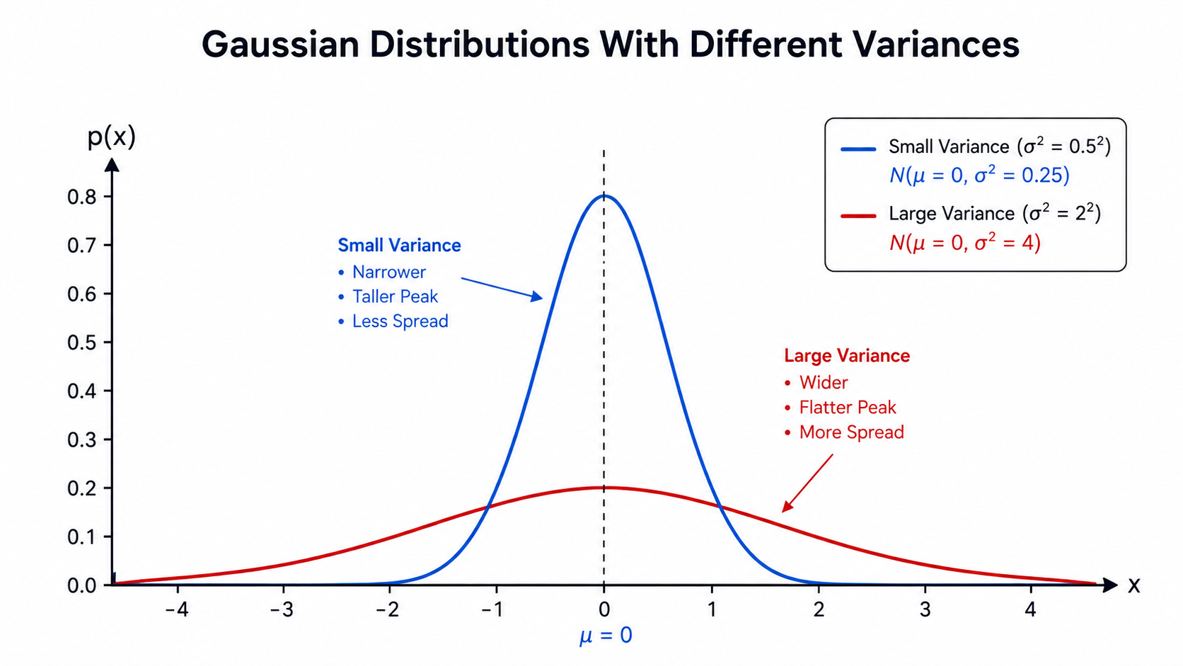
যেখানে: হলো মিন বা গড় (কেন্দ্র) এবং হলো ভ্যারিয়েন্স (ছড়িয়ে থাকা বা spread)।
এটি কেন গুরুত্বপূর্ণ: এই কোর্সের পরের দিকে আপনি যেসব ওয়েট ইনিশিয়ালাইজেশন (weight initialization) স্কিম দেখবেন, সেগুলো খুব সাবধানে বাছাই করা ভ্যারিয়েন্সসহ একটি গাউসিয়ান ডিস্ট্রিবিউশন থেকেই প্রাথমিক ওয়েটগুলো টানে। তাছাড়াও রিগ্রেশনের নয়েজ সম্পর্কে mean squared error লস ঠিক যা ধারণা করে, তা হলো এই গাউসিয়ান ডিস্ট্রিবিউশন, যা আমরা পরের সেকশনে দেখতে পাব।
জয়েন্ট, কন্ডিশনাল প্রোবাবিলিটি এবং বেইজ থিওরেম (Joint, Conditional Probability, and Bayes Theorem)
কোনো দুটি র্যান্ডম ভেরিয়েবল যখন একসাথে ঘটে, তখন তাদের সম্পর্ক বর্ণনা করতে আমাদের আরও কিছু হাতিয়ার দরকার।
যেখানে: হলো জয়েন্ট প্রোবাবিলিটি (A এবং B দুটোই ঘটার সম্ভাবনা), এবং হলো কন্ডিশনাল প্রোবাবিলিটি (B ঘটেছে জানা থাকলে A ঘটার সম্ভাবনা)।
সহজ কথায়: কন্ডিশনাল প্রোবাবিলিটি বলে দেয় যে নতুন তথ্য (B ঘটেছে) জানার পর আমাদের বিশ্বাস কীভাবে বদলে যায়। এটি সম্ভাব্যতার জগতে "যদি...তবে" প্রশ্নের উত্তর।
সহজ কথায়: বেইজ থিওরেম আমাদের একটি কন্ডিশনাল প্রোবাবিলিটিকে তার উল্টো কন্ডিশনাল প্রোবাবিলিটির সাহায্যে ক্যালকুলেট করতে দেয়। এটি নতুন প্রমাণ (evidence) দেখার পর কোনো বিশ্বাসকে (belief) কীভাবে আপডেট করতে হয় তার একটি নীতিবদ্ধ উপায়: P(A) (প্রায়র বা prior বিশ্বাস) থেকে শুরু করে, নতুন ডেটা পর্যবেক্ষণ করার পর P(A|B) (পোস্টেরিয়র বা posterior বিশ্বাস)-এ পৌঁছানো।
এটি কেন গুরুত্বপূর্ণ: যদিও এই কোর্সের নেটওয়ার্কগুলো বেইজিয়ান পদ্ধতিতে সরাসরি ট্রেন করা হয় না, তবুও বেইজ থিওরেমের যুক্তিটি ক্লাসিফায়ারের আউটপুট ব্যাখ্যা করার সময় বারবার ফিরে আসে। একটি ক্লাসিফায়ার মূলত P(class|x) অনুমান করার চেষ্টা করে, এবং এটি বোঝা যে এই সম্ভাবনাটি একটি প্রায়র শ্রেণি-ফ্রিকোয়েন্সি এবং একটি লাইকলিহুড টার্মের সমন্বয়, ইমব্যালান্সড ডেটাসেট (imbalanced dataset) নিয়ে কাজ করার সময় অত্যন্ত সহায়ক।
একটি ধ্রুপদী পরীক্ষা উদাহরণ
ধরি একটি রোগ জনসংখ্যার ১% মানুষের আছে, আর একটি পরীক্ষা ৯৯% সঠিকভাবে শনাক্ত করে কিন্তু ৫% মিথ্যা পজিটিভও দেয়। কারও টেস্ট পজিটিভ এলে তার আসলে রোগ থাকার সম্ভাবনা কত? বেইজ থিওরেম প্রয়োগ করলে দেখা যায় উত্তরটি প্রায় ১৭%, ৯৯% নয়, কারণ প্রায়র প্রোবাবিলিটি (রোগ বিরল হওয়া) হিসাবের ওপর বিশাল প্রভাব ফেলে। এই ধরনের গণনা সচেতনভাবে অভ্যাস করা প্রোবাবিলিস্টিক রিজনিং-এর জন্য চমৎকার একটি ব্যায়াম।
স্বাধীনতা (Independence)
সহজ কথায়: দুটি ঘটনা স্বাধীন হলে একটি সম্পর্কে জানা অন্যটি সম্পর্কে কোনো তথ্য দেয় না। MLE-তে আমরা যখন ধরে নিই যে ট্রেনিং উদাহরণগুলো স্বাধীন এবং অভিন্নভাবে ডিস্ট্রিবিউটেড (independent and identically distributed, বা i.i.d.), তখন এই স্বাধীনতার অনুমানটিই পুরো ডেটাসেটের লাইকলিহুডকে প্রতিটি উদাহরণের লাইকলিহুডের সরল গুণফল হিসেবে লেখার অনুমতি দেয়, যা আমরা একটু পরেই MLE সেকশনে ব্যবহার করব।
এক্সপেকটেশন এবং ভ্যারিয়েন্স (Expectation and Variance)
সহজ কথায়: হলো অনেকবার পুনরাবৃত্তি করার পর পাওয়া -এর দীর্ঘমেয়াদী গড় মান; আর মাপে যে -এর মানগুলো সাধারণত ওই গড়ের চারপাশে কতটা ছড়িয়ে থাকে।
এটি কেন গুরুত্বপূর্ণ: ব্যাচ নরমালাইজেশন (batch normalization) বোঝার জন্য এক্সপেকটেশন এবং ভ্যারিয়েন্স হলো মূল চাবিকাঠি। এটি এমন একটি টেকনিক (যা আপনি পরে দেখবেন), যা প্রতিটি লেয়ারের অ্যাক্টিভেশনগুলোকে এমনভাবে নরমালাইজ করে যেন তাদের মিন (mean) প্রায় শূন্য (zero) এবং ভ্যারিয়েন্স এক (unit) হয়।
হাতে-কলমে উদাহরণ — একটি ন্যায্য পাশার (fair die) এক্সপেকটেশন ও ভ্যারিয়েন্স: একটি ছয়-মুখী পাশার প্রতিটি ফলাফল (1 থেকে 6) সমান সম্ভাব্য, প্রতিটির প্রোবাবিলিটি 1/6।
খেয়াল করুন যে গড় ফলাফল (3.5) আসলে কখনোই পাশা ফেলে সরাসরি পাওয়া যায় না (কারণ পাশার ফলাফল সবসময় পূর্ণসংখ্যা), তবুও এটিই দীর্ঘমেয়াদী গড়। ভ্যারিয়েন্স (প্রায় 2.92) বলে দেয় যে প্রতিটি ফলাফল সাধারণত ওই গড় থেকে মোটামুটি 1.71 এককের মতো দূরে থাকে।
বাস্তব ডেটা থেকে ডেসক্রিপটিভ স্ট্যাটিস্টিকস (Descriptive Statistics From Real Data)
ধরা যাক, আমাদের কাছে একটি নির্দিষ্ট ডেটাসেট আছে। আমরা স্যাম্পল স্ট্যাটিস্টিকস ব্যবহার করে পুরো পপুলেশনের (population) মিন এবং ভ্যারিয়েন্স অনুমান বা এস্টিমেট (estimate) করতে পারি:
এটি কেন গুরুত্বপূর্ণ: ঠিক এই পরিসংখ্যানগুলোই ফিচার স্ট্যান্ডার্ডাইজেশনের (feature standardization) সময় (যা একটি খুব সাধারণ প্রিপ্রসেসিং ধাপ) প্রতিটি ফিচারের জন্য, এবং ব্যাচ নরমালাইজেশন লেয়ারের ভেতরে প্রতি ব্যাচের জন্য ক্যালকুলেট করা হয়।
হাতে-কলমে উদাহরণ: মানগুলো থাকা একটি ফিচারের জন্য:
স্ট্যান্ডার্ডাইজ করা মানগুলো হলো — যাদের মিন 0, ভ্যারিয়েন্স 1, যা ট্রেনিংয়ের আগে কোনো ফিচারকে স্ট্যান্ডার্ডাইজ করার মূল লক্ষ্য।
ম্যাক্সিমাম লাইকলিহুড এস্টিমেশন: লস ফাংশনগুলো আসলে যেখান থেকে আসে (Maximum Likelihood Estimation: Where Loss Functions Actually Come From)
এই চ্যাপ্টারের সবচেয়ে বড় প্রাপ্তি হলো এটি — আমরা নির্দিষ্ট কিছু লস ফাংশন কেন ব্যবহার করি, তার উত্তর লুকিয়ে আছে এখানেই।
ধরা যাক, একটি মডেল সম্ভাব্য আউটপুটগুলোর ওপর একটি প্রোবাবিলিটি ডিস্ট্রিবিউশন সংজ্ঞায়িত করে এবং আমাদের কাছে একটি ট্রেনিং ডেটাসেট আছে। Maximum Likelihood Estimation এমন সব প্যারামিটার -কে বেছে নেয়, যা মডেলটিকে আমাদের বাস্তবে দেখা বা পর্যবেক্ষণ করা ডেটার জন্য সবচেয়ে বেশি প্রোবাবিলিটি বা সম্ভাবনা দিতে সাহায্য করে।
সহজ কথায়: -এর সম্ভাব্য সমস্ত সেটিংসের মধ্যে থেকে এমন একটিকে বেছে নিন, যার অধীনে আপনি বাস্তবে যে ট্রেনিং ডেটা সংগ্রহ করেছেন তা ঘটার সম্ভাবনা সবচেয়ে কম বিস্ময়কর (least surprising) হতো।
একেবারে গোড়া থেকে বাইনারি ক্রস-এন্ট্রপি প্রতিপাদন করা (Deriving binary cross-entropy from scratch)। ধরা যাক, মডেলটি আউটপুট দেয়, যাকে একটি বার্নোলি প্রোবাবিলিটি হিসেবে ব্যাখ্যা করা হয়। সংখ্যক স্বাধীন (independent) ট্রেনিং উদাহরণের জন্য, পুরো ট্রেনিং সেটের লাইকলিহুড হলো:
অনেকগুলো ছোট ছোট প্রোবাবিলিটিকে একসাথে গুণ করলে তা নিউমেরিক্যালি শূন্যের দিকে আন্ডারফ্লো (underflow) করে, তাই এর বদলে আমরা লগ (log)-লাইকলিহুডকে ম্যাক্সিমাইজ করি — লগারিদম যেহেতু সবসময়েই বাড়তে থাকে (monotonically increasing), তাই এটি একই ম্যাক্সিমাইজার বা সর্বোচ্চ মান দেয়:
সবশেষে, যেহেতু অপ্টিমাইজেশনকে সাধারণত লস কমানোর (minimizing) বিষয় হিসেবে দেখা হয়, তাই আমরা একে নেগেটিভ বা ঋণাত্মক করি এবং সংখ্যক উদাহরণের ওপর গড় করি — আর এটি ঠিক হুবহু বাইনারি ক্রস-এন্ট্রপি তৈরি করে:
পুরো বড় ছবিটা (The big picture)
Cross-entropy লস মিনিমাইজ করা এবং একটি বার্নোলি (বা মাল্টি-ক্লাস প্রবলেমের ক্ষেত্রে ক্যাটাগরিক্যাল) মডেলের অধীনে ট্রেনিং ডেটার লাইকলিহুড ম্যাক্সিমাইজ করা — গাণিতিকভাবে এই দুটি সম্পূর্ণ এক। এটি কোনো কাকতালীয় ব্যাপার বা মনগড়া কনভেনশন নয় — মডেলের আউটপুটটি একটি প্রকৃত প্রোবাবিলিটি, এই অনুমানের ওপর ভিত্তি করে MLE ঠিক যে লস ফাংশনটি প্রতিপাদন করে তা হলো cross-entropy। ঠিক একই ধরনের প্রতিপাদন, তবে বার্নোলির বদলে গাউসিয়ান নয়েজ ধরে নিয়ে করলে, তা রিগ্রেশনের জন্য mean squared error তৈরি করে — কোর্সের পরের দিকের একটি নির্দিষ্ট লস-ফাংশন চ্যাপ্টারে আপনি এর সম্পূর্ণ বিস্তারিত রূপ দেখতে পাবেন।
গ্র্যাজুয়েট-লেভেলে প্রায়ই জিজ্ঞেস করা একটি প্রশ্ন
"একেবারে মূল বা ফার্স্ট প্রিন্সিপালস (first principles) থেকে cross-entropy loss প্রতিপাদন করো।" উপরের ধাপগুলো পুনরায় অনুসরণ করুন: পুরো ডেটাসেটের বার্নোলি লাইকলিহুড থেকে শুরু করুন, এর লগারিদম নিন, এটিকে নেগেটিভ করুন এবং গড় বের করুন। এটি মুখস্থ থেকে নিজে নিজে ধাপে ধাপে করে দেখাতে পারাটা আপনার প্রকৃত বোঝাপড়ার প্রমাণ দেয়, শুধু সূত্র মুখস্থ করার নয়।
এনট্রপি এবং KL ডাইভারজেন্স: ক্রস-এন্ট্রপির আরেকটি দৃষ্টিকোণ (Entropy and KL Divergence: Another View of Cross-Entropy)
আমরা ইতিমধ্যে দেখেছি যে cross-entropy loss MLE থেকে সরাসরি বেরিয়ে আসে। কিন্তু একই সূত্রটির আরেকটি চমৎকার ব্যাখ্যা আছে, যা তথ্য তত্ত্ব বা ইনফরমেশন থিওরি (information theory) থেকে আসে।
সহজ কথায়: এনট্রপি মাপে একটি ডিস্ট্রিবিউশনে কতটা অনিশ্চয়তা বা এলোমেলোভাবে বিস্তৃত তথ্য আছে। একটি ফলাফল প্রায় নিশ্চিত হলে (যেমন P(x=1)=0.99) এনট্রপি কম হয়; সব ফলাফল সমান সম্ভাব্য হলে (যেমন একটি ন্যায্য কয়েন) এনট্রপি সর্বোচ্চ হয়।
যেখানে: হলো আসল বা ট্রু ডিস্ট্রিবিউশন (যেমন, ট্রেনিং লেবেলের ওয়ান-হট ডিস্ট্রিবিউশন), হলো মডেলের প্রেডিক্ট করা ডিস্ট্রিবিউশন, এবং হলো Kullback-Leibler ডাইভারজেন্স, যা মাপে Q, P থেকে কতটা দূরে আছে।
সহজ কথায়: cross-entropy H(P,Q) সবসময় এনট্রপি H(P)-এর চেয়ে বড় বা সমান, আর এই পার্থক্যটাই হলো KL ডাইভারজেন্স, অর্থাৎ মডেলের ডিস্ট্রিবিউশন সত্যিকারের ডিস্ট্রিবিউশন থেকে কতটা দূরে আছে তার একটি পরিমাপ। যেহেতু ট্রেনিং ডেটার P ফিক্সড বা স্থির থাকে, তাই cross-entropy কমানো এবং KL ডাইভারজেন্স কমানো একই কাজ। অর্থাৎ, cross-entropy loss মিনিমাইজ করার মানে হলো মডেলের প্রেডিকশন ডিস্ট্রিবিউশনকে ট্রু ডিস্ট্রিবিউশনের যতটা সম্ভব কাছাকাছি নিয়ে আসা।
একই গন্তব্যে দুটি পথ
MLE-এর দৃষ্টিকোণ (লাইকলিহুড ম্যাক্সিমাইজ করা) এবং ইনফরমেশন থিওরির দৃষ্টিকোণ (KL ডাইভারজেন্স মিনিমাইজ করা), এই দুটোই গাণিতিকভাবে একদম হুবহু একই অপ্টিমাইজেশন সমস্যায় গিয়ে পৌঁছায়। এটি আরেকবার নিশ্চিত করে যে cross-entropy loss কোনো স্বেচ্ছাচারী পছন্দ নয়, বরং একাধিক স্বাধীন গাণিতিক পথ থেকেই এটি প্রাকৃতিকভাবে বেরিয়ে আসে।
Implementation
python
স্ট্যান্ডার্ডাইজেশন ব্লকটি হাতে করা হিসেবটিকে পুনরায় করে দেখায় এবং এটি নিশ্চিত করে যে numpy-এর mean() এবং var() উপরের ম্যানুয়াল পাটিগণিতের সাথে হুবহু মিলে যায়। ক্রস-এন্ট্রপি ব্লকটি এই চ্যাপ্টারে প্রতিপাদন করা সূত্রটিকে সরাসরি ইমপ্লিমেন্ট করে: প্রতিটি উদাহরণের জন্য, আসল লেবেল 1 হলে এটি নেয় এবং 0 হলে নেয়, তারপর পুরো ব্যাচের ওপর গড় করে — এটি ঠিক হুবহু আমাদের প্রতিপাদন করা সেই নেগেটিভ করা এবং গড় করা লগ-লাইকলিহুড।
log(0) থেকে সাবধান
যদি একটি প্রেডিক্ট করা প্রোবাবিলিটি কখনো হুবহু 0 বা 1 হয়ে যায়, তবে np.log -inf অথবা একটি ওয়ার্নিং তৈরি করবে এবং লসটি nan হয়ে যেতে পারে। প্রোডাকশন ইমপ্লিমেন্টেশনগুলো লগারিদম নেওয়ার আগে প্রেডিকশনগুলোকে 0 এবং 1-এর খুব কাছাকাছি একটি ছোট এপসিলন (epsilon) দূরত্বে আটকে দেয় বা ক্লিপ করে (যেমন np.clip(y_pred, 1e-7, 1-1e-7))।
মূল বিষয়গুলো (Key Takeaways)
Key Takeaways
- বার্নোলি (Bernoulli) এবং ক্যাটাগরিক্যাল (Categorical) ডিস্ট্রিবিউশন যথাক্রমে বাইনারি এবং মাল্টি-ক্লাস ক্লাসিফিকেশন আউটপুটগুলোকে মডেল করে; গাউসিয়ান (Gaussian) ডিস্ট্রিবিউশন ওয়েট ইনিশিয়ালাইজেশন এবং mean squared error লসের মূল ভিত্তি তৈরি করে।
- এক্সপেকটেশন (Expectation) কোনো ডিস্ট্রিবিউশনের গড় মান পরিমাপ করে; ভ্যারিয়েন্স (variance) মাপে ওই গড়ের চারপাশে কতটা ছড়িয়ে আছে।
- স্যাম্পল মিন এবং ভ্যারিয়েন্স (যা বাস্তব ডেটা থেকে ক্যালকুলেট করা হয়) ফিচার স্ট্যান্ডার্ডাইজেশনে এবং ব্যাচ নরমালাইজেশন লেয়ারের ভেতরে ব্যবহার করা হয়।
- Cross-entropy loss কোনো মনগড়া পছন্দ নয় — এটি একটি বার্নোলি বা ক্যাটাগরিক্যাল আউটপুট অনুমানের অধীনে Maximum Likelihood Estimation-এর সরাসরি গাণিতিক ফলাফল।
- ঠিক একই MLE যুক্তি যদি বার্নোলির বদলে একটি গাউসিয়ান নয়েজ অনুমানের ওপর প্রয়োগ করা হয়, তবে তা রিগ্রেশনের জন্য mean squared error loss তৈরি করে।
সাধারণ ভুল ধারণা (Common Mistakes)
cross-entropy এবং MSE-কে মনগড়া কনভেনশন হিসেবে ধরে নেওয়া
কোনো ব্যাখ্যা ছাড়াই একটি সাধারণ নিয়ম হিসেবে "ক্লাসিফিকেশনের জন্য cross-entropy, রিগ্রেশনের জন্য MSE" মুখস্থ করে ফেলাটা খুব সহজ। কিন্তু এই দুটোই হলো আউটপুটের ওপর করা একটি নির্দিষ্ট প্রোবাবিলিস্টিক বা সম্ভাব্যতামূলক অনুমানের (বার্নোলি/ক্যাটাগরিক্যাল বনাম গাউসিয়ান) সাথে Maximum Likelihood Estimation যুক্ত হওয়ার সরাসরি ফলাফল — এটি বুঝতে পারলে, যেসব ডিস্ট্রিবিউশন এই দুটির কোনো ছাঁচেই পড়ে না তাদের জন্য কোন লস ব্যবহার করতে হবে তা আপনি নিজেই যুক্তি দিয়ে বুঝতে পারবেন।
পপুলেশন ভ্যারিয়েন্সের সাথে স্যাম্পল ভ্যারিয়েন্স গুলিয়ে ফেলা
দিয়ে ভাগ করা (পপুলেশন ভ্যারিয়েন্স) এবং দিয়ে ভাগ করা (আনবায়াসড বা নিরপেক্ষ স্যাম্পল ভ্যারিয়েন্স এস্টিমেটর, যাকে বেসেলের কারেকশন বা Bessel's correction বলে)-এর মধ্যে সামান্য পার্থক্য থাকে। আপনি ddof=1 পাস না করলে NumPy-এর .var() সাধারণত ডিফল্টভাবে দিয়ে ভাগ করে। বড় ব্যাচের ক্ষেত্রে এটি খুব একটা প্রভাব ফেলে না, কিন্তু ছোটখাটো নিউমেরিক্যাল পার্থক্যের এটি একটি সাধারণ কারণ।
বেইজ থিওরেমে প্রায়র উপেক্ষা করা
বিরল ঘটনার (rare event) ক্ষেত্রে P(A|B) হিসাব করার সময় শুধু P(B|A)-এর ওপর ভিত্তি করে সিদ্ধান্ত নেওয়া একটি সাধারণ ভুল। একটি টেস্ট ৯৯% নির্ভুল হলেও, ঘটনাটি নিজে যদি অত্যন্ত বিরল হয় (কম প্রায়র), তবে পজিটিভ ফলাফলের পরও প্রকৃতপক্ষে ঘটনা ঘটার সম্ভাবনা অনেক কম হতে পারে। সবসময় প্রায়র প্রোবাবিলিটিকে হিসাবের মধ্যে রাখতে হবে।
এনট্রপি এবং cross-entropy-কে একই জিনিস ভেবে নেওয়া
এনট্রপি H(P) শুধু একটি ডিস্ট্রিবিউশনের নিজস্ব অনিশ্চয়তা মাপে, কিন্তু cross-entropy H(P,Q) দুটি ভিন্ন ডিস্ট্রিবিউশনের (আসল এবং প্রেডিক্ট করা) মধ্যেকার সম্পর্ক মাপে। যখন P এবং Q একই হয়, তখনই কেবল cross-entropy এনট্রপির সমান হয়ে যায়; অন্য সব ক্ষেত্রে cross-entropy সবসময় এনট্রপির চেয়ে বড় হবে।
ইন্টারভিউ কর্নার (Interview Corner)
Quick Check
বাস্তবে এটি কোথায় দেখা যায় (Where This Shows Up in Practice)
প্রতিটি ক্লাসিফায়ারের কনফিডেন্স স্কোর (confidence score), ব্যাচ নরমালাইজেশনের প্রতিটি ব্যবহার, এবং এই পুরো কোর্সের লস ফাংশনের প্রতিটি বাছাই সরাসরি এই চ্যাপ্টারের ধারণাগুলোতেই ফিরে যায়। ভেক্টর ও ম্যাট্রিক্স (স্ট্রাকচার বা গঠন বর্ণনা করে), ক্যালকুলাস (কীভাবে শিখতে হবে তা বর্ণনা করে) এবং প্রোবাবিলিটি (একটি লস ফাংশন আসলে কী বোঝায় তা বর্ণনা করে) — এই সবকিছু এক জায়গায় হওয়ার পর, এখন আপনার কাছে লেয়ারের পর লেয়ার ধরে খুব নিখুঁতভাবে backpropagation প্রতিপাদন করার জন্য প্রয়োজনীয় সম্পূর্ণ গাণিতিক ভিত্তি প্রস্তুত আছে — আর কোর্সটি এরপর ঠিক ওই জায়গাতেই যাবে।