Chapter 19 of 25
Regularization
Keeping a network from memorizing instead of learning
19 min read
Created ২ আগ, ২০২৬
ভূমিকা (Motivation)
ধরুন, একজন ছাত্র গত বছরের পরীক্ষার প্রশ্ন ও উত্তর হুবহু মুখস্থ করে গেল। সে হয়তো ওই নির্দিষ্ট পরীক্ষাতে খুব দারুণ রেজাল্ট করবে — কিন্তু এই বছরের পরীক্ষায় যখনই একই বিষয়ের ওপর একটু ঘুরিয়ে প্রশ্ন করা হবে, তখনই সে খুব বাজেভাবে ফেল করবে। সে আসলে বিষয়টি শেখেনি; সে শিখেছে ওই প্রশ্নের উত্তরগুলো। একটি নিউরাল নেটওয়ার্কও ঠিক একই ফাঁদে পা দিতে পারে: যদি তার শেখার ধারণক্ষমতা বা ক্যাপাসিটি অনেক বেশি হয়, তবে সে পুরো ট্রেনিং সেটটিকেই (training set) — যার মধ্যে থাকা নয়েজ (noise), ছোটখাটো খামখেয়ালিপনা বা কাকতালীয় বিষয়গুলোও বাদ যায় না — এতটাই ভালোভাবে মুখস্থ করে ফেলতে পারে যে ট্রেনিং লস (training loss) প্রায় শূন্যের কাছাকাছি চলে যায়, অথচ সে এমন কিছুই শেখে না যা নতুন ডেটার ওপর প্রয়োগ করা বা জেনারেলাইজ (generalize) করা যায়।
রেগুলারাইজেশন (Regularization) হলো এমন সব কৌশলের একটি ছাতা বা সাধারণ নাম, যা ঠিক এই প্রবণতাটির বিরুদ্ধে লড়াই করে — যা একটি নেটওয়ার্ককে নির্দিষ্ট উদাহরণ মুখস্থ করার বদলে আসল প্যাটার্ন শিখতে উৎসাহ দেয় বা বাধ্য করে। যেহেতু MLP-গুলোর, বিশেষ করে ডিপ (deep) এবং চওড়া বা ওয়াইড (wide) MLP-গুলোর, মুখস্থ করার raw ক্ষমতা বা ধারণক্ষমতা থাকে প্রচুর, তাই রেগুলারাইজেশন কোনো ঐচ্ছিক বা অপশনাল জিনিস নয়; বাস্তবে প্রায় প্রতিটি ট্রেনিং রান-এই এটি ব্যবহার করা হয়।
একটি বাস্তব জীবনের উদাহরণ (A Real-Life Scenario)
ভাবুন তো, একটি হাসপাতাল রোগীদের ল্যাব রিপোর্ট থেকে তাদের ঝুঁকি প্রেডিক্ট বা অনুমান করার জন্য একটি মডেল ট্রেন করছে। যথেষ্ট পরিমাণ হিডেন ইউনিট (hidden units) থাকলে, নেটওয়ার্কটি এতটাই শক্তিশালী হতে পারে যে সে কার্যত প্রতিটি ট্রেনিং রোগীর জন্য ভেতরে একটি নিজস্ব "ফিঙ্গারপ্রিন্ট" বা আঙুলের ছাপ তৈরি করে এবং সহজভাবে তাদের ফলাফলটি মুখস্থ করে ফেলে — আর এর মধ্যে এমন সব খামখেয়ালিপনা বা নয়েজও ঢুকে যায় যার সাথে আসল ঝুঁকির কোনো সম্পর্কই নেই, যেমন হয়তো কোনো নির্দিষ্ট দিনে একটি নির্দিষ্ট ল্যাব মেশিনের রাউন্ডিংয়ের (rounding) অভ্যাস। ট্রেনিং সেটের ওপর, এই মডেলটিকে নিখুঁত বলে মনে হয়। কিন্তু পরের মাসে যখন নতুন রোগীদের ওপর এটি প্রয়োগ করা হয়, তখন এর পারফরম্যান্স একটি কয়েন টস করার চেয়ে খুব একটা ভালো হয় না, কারণ এটি কখনোই ল্যাবের ভ্যালু এবং ঝুঁকির মধ্যে থাকা আসল মেডিকেল সম্পর্কটি শেখেনি — এটি মূলত একটি লুকআপ টেবিল (lookup table) বা ডিকশনারি শিখেছে।
রেগুলারাইজেশন হলো সেই জিনিস যা ওই হাসপাতালের মডেলটিকে সৎ রাখে: এটি মডেলটিকে ঠিক ততটাই বেঁধে রাখে বা সীমাবদ্ধ করে যাতে শুধু নয়েজ মুখস্থ করাটা একটি ব্যর্থ কৌশল হয়ে দাঁড়ায়, আর আসল ভেতরের সিগন্যালটি (signal) শেখাটা একটি সফল কৌশল হিসেবে টিকে থাকে।
মূল ধারণা তৈরি করা (Building the Intuition)
যেকোনো ফর্মুলা দেখার আগেই, এই চ্যাপ্টারের প্রতিটি কৌশলের বা টেকনিকের মধ্যে দিয়ে বয়ে চলা মূল থিমটি বা কথাটি জেনে নিন:
- ওভারফিটিং (Overfitting) তখনই ঘটে যখন একটি মডেল ডেটার মধ্যে থাকা আসল সিগন্যালের প্রয়োজনের চেয়ে বেশি স্বাধীনতা বা ফ্রিডম (freedom) পায়, তাই সে ওই বাড়তি স্বাধীনতাটুকু খরচ করে নয়েজের সাথে ফিট (fit) হতে।
- প্রায় প্রতিটি রেগুলারাইজেশন টেকনিকই কাজ করে মডেলের কাছ থেকে ওই স্বাধীনতাটুকু কিছুটা কেড়ে নেওয়ার মাধ্যমে — সেটি বড় ওয়েটগুলোকে (weights) শাস্তি বা পেনাল্টি (penalty) দিয়ে হতে পারে, নেটওয়ার্কের বিভিন্ন অংশকে র্যান্ডম বা দৈবভাবে অকেজো করে হতে পারে, মডেলের মুখস্থ করার সময় পাওয়ার আগেই ট্রেনিং থামিয়ে দিয়ে হতে পারে, অথবা ট্রেনিংয়ের ভেতরেই কিছুটা নয়েজ বা গোলমাল ঢুকিয়ে দিয়ে হতে পারে।
- এই কৌশলগুলোর কোনোটিই একটি নেটওয়ার্কের ভেতরে থাকা মৌলিক শেখার ক্ষমতাকে বা কী শিখতে সক্ষম তা পরিবর্তন করে না — এগুলো শুধু একটি নির্দিষ্ট পরিমাণ ট্রেনিং ডেটা ও সময়ের সাপেক্ষে নেটওয়ার্কটিকে আসলে কী শিখতে উৎসাহিত করা হচ্ছে, সেটি পরিবর্তন করে।
এল১ এবং এল২ রেগুলারাইজেশন (L1 and L2 Regularization)
একটি নেটওয়ার্কের স্বাধীনতা কমানোর সবচেয়ে সরাসরি উপায় হলো লস ফাংশনের (loss function) ঠিক ভেতরেই ওয়েটগুলোকে শাস্তি বা পেনাল্টি দেওয়া।
যেখানে: হলো রেগুলারাইজেশনের শক্তি বা স্ট্রেন্থ (এটি একটি হাইপারপ্যারামিটার যা আপনাকে বেছে নিতে হয়), এবং হলো ওয়েট ম্যাট্রিক্সের স্কয়ারড এল২ নর্ম (squared L2 norm)।
গ্রেডিয়েন্টের ওপর প্রভাব: পেনাল্টি টার্মটিকে ডিফারেনসিয়েট (differentiate) করলে গ্রেডিয়েন্টের সাথে একটি অতিরিক্ত যোগ হয়, যা আপডেটটিকে এমনভাবে বদলে দেয়: । প্রতিটি পদক্ষেপে প্রতিটি ওয়েট একটি নির্দিষ্ট অনুপাতে বা গুণগতভাবে শূন্যের দিকে কিছুটা ছোট হয়ে যায় — আর ঠিক এই কারণেই এর নাম দেওয়া হয়েছে ওয়েট ডিকে (weight decay)।
এল২ (L2) থেকে এর মূল পার্থক্য: প্রতিটি ওয়েটের সাপেক্ষে L1-এর গ্রেডিয়ent হলো একটি কনস্ট্যান্ট বা ধ্রুবক (শুধু ওয়েটটির সাইন বা চিহ্ন), ওয়েটের আকার বা ম্যাগনিটিউড (magnitude) যাই হোক না কেন — যেখানে L2-এর গ্রেডিয়েন্ট ওয়েটের ম্যাগনিটিউডের সমানুপাতিক। ওই কনস্ট্যান্ট বা ধ্রুবক ধাক্কাটি এতটাই শক্তিশালী যে তা অনেক ওয়েটকে পুরোপুরি ঠিক শূন্যতে নামিয়ে আনতে পারে, যার ফলে স্পার্স (sparse) বা পাতলা ওয়েট ম্যাট্রিক্স তৈরি হয়, যেখানে L2-এর সমানুপাতিক ধাক্কা ওয়েটগুলোকে মসৃণভাবে শূন্যের দিকে ছোট করে ঠিকই, কিন্তু খুব কম সময়েই তা ঠিক শূন্যতে পৌঁছায়।
ইলাস্টিক নেট (Elastic Net): এক ঢিলে দুই পাখি মারা
ইলাস্টিক নেট এই দুটি পেনাল্টিকেই এক করে ফেলে: , যার লক্ষ্য হলো L1-এর স্পার্স বা পাতলা করার ক্ষমতা এবং L2-এর আরও মসৃণ ও স্থিতিশীলভাবে ছোট করার ক্ষমতা — এই দুটোকেই একসাথে কাজে লাগানো।
| বিষয় (Aspect) | এল১ (L1) | এল২ (L2) |
|---|---|---|
| ওয়েটের ওপর প্রভাব | অনেক ওয়েটকে ঠিক শূন্যতে নামিয়ে আনে (স্পার্সিটি) | সব ওয়েটকে মসৃণভাবে ছোট করে, খুব কম সময়ই ঠিক শূন্যতে নামায় |
| ব্যাখ্যা (Interpretation) | ইমপ্লিসিট ফিচার সিলেকশন (Implicit feature selection) | কমপ্লেক্সিটি বা জটিলতার মসৃণ নিয়ন্ত্রণ |
| গ্রেডিয়েন্ট (Gradient) | কনস্ট্যান্ট বা স্থির ম্যাগনিটিউড (±λ) | ওয়েটের ম্যাগনিটিউডের সমানুপাতিক |
| সাধারণ ব্যবহার | যখন একটি স্পার্স (sparse) এবং সহজে ব্যাখ্যা করা যায় এমন মডেল দরকার হয় | MLP-র জন্য ডিফল্ট বা সাধারণ-উদ্দেশ্যে সবচেয়ে ভালো পছন্দ |
হাতে-কলমে উদাহরণ: L2 ওয়েট ডিকে সংখ্যাগতভাবে (Worked Example: L2 Weight Decay Numerically)
ধরুন একটি ওয়েট , লার্নিং রেট , এবং রেগুলারাইজেশন শক্তি । তাহলে আপডেট রুল অনুযায়ী, শুধু ডিকে অংশটি প্রয়োগ করলে (ডেটা গ্রেডিয়েন্ট সাময়িকভাবে শূন্য ধরে) প্রতিটি ধাপে:
অর্থাৎ প্রতিটি ধাপে ওয়েটটি তার আগের মানের ৯৯.৯% হয়ে যায়। ১০০০ ধাপ পর, যদি ডেটা গ্রেডিয়েন্ট থেকে কোনো প্রতিরোধ না থাকত, তবে কমে দাঁড়াত -এ — প্রায় অর্ধেকের বেশি সংকুচিত। বাস্তবে অবশ্য ডেটা গ্রেডিয়েন্ট প্রতিনিয়ত এই সংকোচনের বিরুদ্ধে লড়াই করে, তাই ওয়েটটি শূন্যে চলে যায় না, বরং এমন একটি ভারসাম্য বিন্দুতে গিয়ে স্থির হয় যেখানে ডেটার প্রয়োজনীয়তা এবং ডিকের চাপ একে অপরকে সমান করে দেয় — এটাই হলো L2 রেগুলারাইজেশনের আসল কাজের প্রক্রিয়া।
L1, L2 এবং ড্রপআউট: কখন কোনটি বেছে নেবেন (Choosing Between L1, L2, and Dropout)
| পরিস্থিতি (Situation) | সবচেয়ে ভালো পছন্দ (Best Choice) | কারণ (Why) |
|---|---|---|
| একটি সাধারণ-উদ্দেশ্যে MLP, বিশেষ কারণ ছাড়া | L2 / ওয়েট ডিকে | মসৃণ, স্থিতিশীল, এবং প্রায় সবসময় নিরাপদ ডিফল্ট |
| ফিচার সিলেকশন বা কোন ইনপুটগুলো গুরুত্বপূর্ণ তা জানার দরকার | L1 | স্পার্সিটি তৈরি করে, অপ্রয়োজনীয় ওয়েটকে ঠিক শূন্যে নামায় |
| খুব বড় এবং গভীর নেটওয়ার্ক, প্রচুর প্যারামিটার | ড্রপআউট (L2-এর সাথে মিলিয়ে) | কো-অ্যাডাপ্টেশন আটকায়, যা শুধু ওয়েট ছোট করে সমাধান হয় না |
| ছোট ডেটাসেট, দ্রুত ওভারফিট হওয়ার ঝুঁকি | L2 + আর্লি স্টপিং | শক্তিশালী ড্রপআউট রেট ছোট ডেটাসেটে ট্রেনিংকে অস্থির করতে পারে |
ড্রপআউট (Dropout)
সংজ্ঞা (Definition)
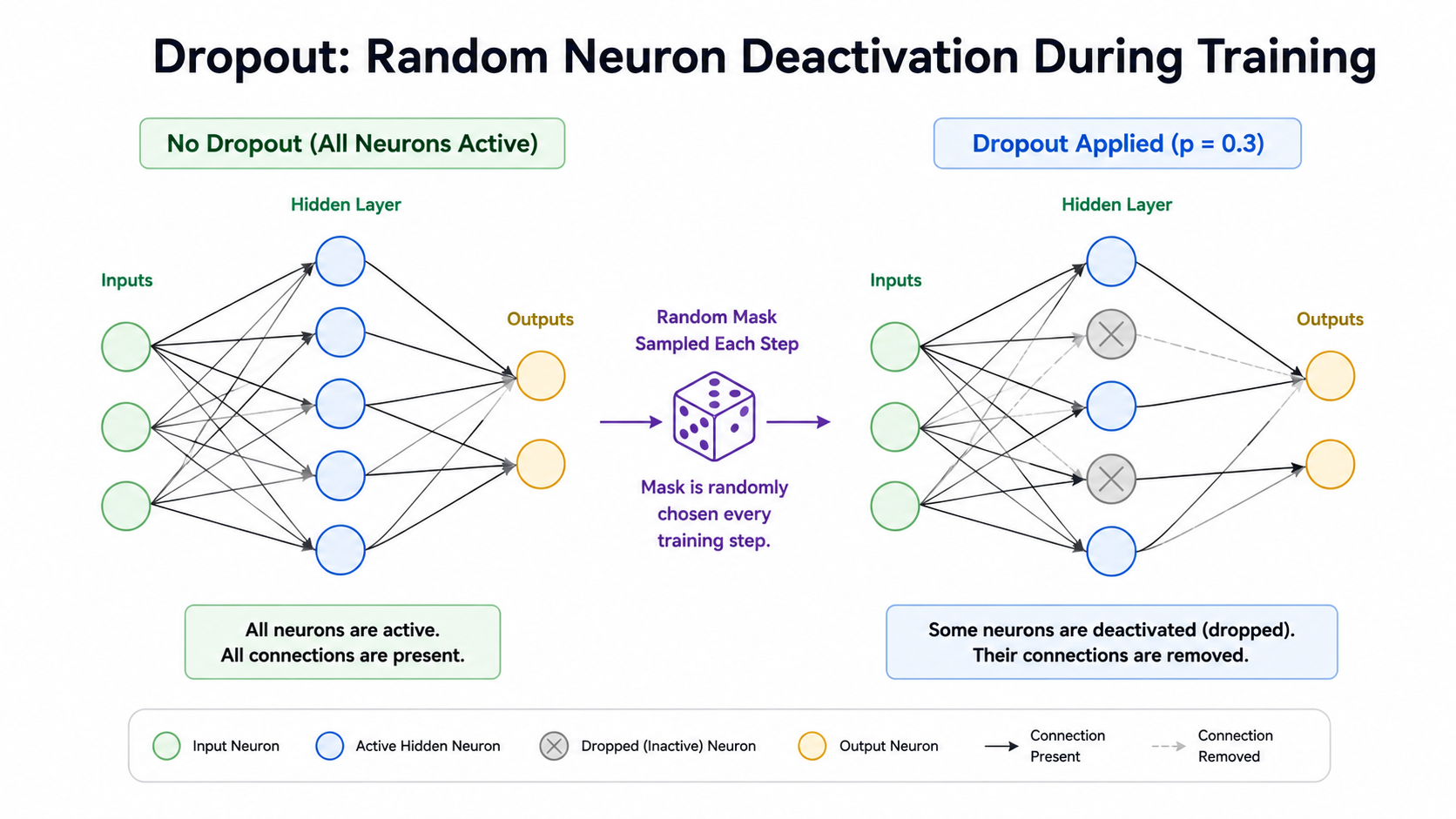
ড্রপআউট হলো এমন একটি রেগুলারাইজেশন টেকনিক যা প্রতিটি ট্রেনিং ধাপের সময় প্রতিটি নিউরনের অ্যাক্টিভেশনকে সম্ভাবনার (probability) সাথে (সাধারণত ০.২ থেকে ০.৫) র্যান্ডমভাবে "ড্রপ (drop)" করে বা শূন্য করে দেয় — এবং প্রতিটি নিউরন ও প্রতিটি ট্রেনিং এক্সাম্পলের জন্য এই কাজটি স্বাধীনভাবে বা ইনডিপেনডেন্টলি করা হয়।
ট্রেনিংয়ের সময়:
ইনফারেন্সের (inference) সময়: কোনো ড্রপআউট প্রয়োগ করা হয় না — নেটওয়ার্ক আগের মতোই স্বাভাবিকভাবে তার সব নিউরন ব্যবহার করে। ট্রেনিংয়ের সময় এই দিয়ে ভাগ করার কারণে ("ইনভার্টেড ড্রপআউট") ট্রেনিং এবং ইনফারেন্সের সময় অ্যাক্টিভেশনের এক্সপেক্টেড ম্যাগনিটিউড বা প্রত্যাশিত মাত্রা স্বয়ংক্রিয়ভাবে সমান হয়ে যায়, তাই টেস্টের সময় কোনো রিক্যালকুলেশন বা রিস্কেলিংয়ের (rescaling) দরকার হয় না।
ড্রপআউট কেন কাজ করে — দুটি পরিপূরক ধারণা
(১) কো-অ্যাডাপ্টেশন বা পরস্পরের ওপর নির্ভরশীল হওয়া আটকানো: ড্রপআউট ছাড়া, নিউরনগুলো খুব সহজেই নির্দিষ্ট কোনো অন্য নিউরনের উপস্থিতির ওপর অতিরিক্ত নির্ভরশীল হয়ে পড়তে পারে, যার ফলে খুব ঠুনকো, কো-ডিপেন্ডেন্ট বা পরস্পরের ওপর নির্ভরশীল ফিচার তৈরি হয়। ড্রপআউট প্রতিটি নিউরনকে অন্য নিউরনগুলোর বিভিন্ন র্যান্ডম সাবসেটের (random subsets) উপস্থিতিতেও দরকারী থাকতে বাধ্য করে, যা অনেক বেশি শক্তিশালী এবং স্বাধীনভাবে অর্থপূর্ণ ফিচার তৈরি করতে উৎসাহিত করে।
(২) ইমপ্লিসিট এনসেম্বলিং (Implicit ensembling): ড্রপআউট দিয়ে ট্রেন করাকে মূলত একই সাথে অসংখ্য ভিন্ন ভিন্ন "পাতলা বা thinned" সাব-নেটওয়ার্ক ট্রেন করার মতো করে দেখা যেতে পারে — যেখানে প্রতিটি র্যান্ডম মাস্ক (random mask) একটি আলাদা সাব-নেটওয়ার্ক তৈরি করে — যারা সবাই একই ওয়েটস শেয়ার করে, এবং চূড়ান্ত ট্রেন হওয়া নেটওয়ার্কটি এদের সবার একটি গড়ের বা অ্যাভারেজের (average) মতো আচরণ করে। এনসেম্বল (Ensemble) বা অনেকগুলো মডেলের সমষ্টি যেকোনো একটি একক মডেলের চেয়ে ভালো জেনারেলাইজ করতে পারে বলে পরিচিত, আর ড্রপআউট কার্যত প্রায় বিনামূল্যে সেই সুবিধাটির বেশিরভাগই এনে দেয়।
ড্রপআউটের সবচেয়ে সাধারণ বাগ বা ভুল (The most common dropout bug)
ইনফারেন্স বা ইভ্যালুয়েশনের (evaluation) সময় ড্রপআউট বন্ধ করতে ভুলে গেলে (অথবা ট্রেনিংয়ের সময় ওই রিস্কেলিংটি ভুলে গেলে) ট্রেনিংয়ের সময়কার অ্যাক্টিভেশন ম্যাগনিটিউড এবং টেস্টের সময়কার অ্যাক্টিভেশন ম্যাগনিটিউডের মধ্যে একটি বড় অমিল তৈরি হয়, যা মডেলের পারফরম্যান্সকে নীরবে ধ্বংস করে দেয়। ফ্রেমওয়ার্কগুলো model.eval() (PyTorch) অথবা training=False (Keras) মোড ফ্ল্যাগ দিয়ে এটি স্বয়ংক্রিয়ভাবে সামলে নেয় — তাই ইভ্যালুয়েশনের আগে সবসময় নিশ্চিত হয়ে নিন যে এটি ঠিকমতো সেট করা আছে কি না।
আর্লি স্টপিং (Early Stopping)
সংজ্ঞা (Definition)
আর্লি স্টপিং ট্রেনিংয়ের সময় আলাদা করে সরিয়ে রাখা একটি ভ্যালিডেশন সেটের (validation set) ওপর মডেলের পারফরম্যান্সের দিকে নজর রাখে, এবং যখনই নির্দিষ্ট সংখ্যক ইপক (epoch) ধরে (যাকে "পেশেন্স বা patience" বলা হয়) ভ্যালিডেশন পারফরম্যান্স আর ভালো হয় না, তখন এটি ট্রেনিং থামিয়ে দেয়, এমনকি যদি ট্রেনিং লস তখনও কমতে থাকে তবুও।
এটি সরাসরি ক্লাসিক ওভারফিটিংয়ের লক্ষণটিকে টার্গেট করে: যখন ট্রেনিং লস কমতেই থাকে কিন্তু ভ্যালিডেশন লস উল্টো আবার বাড়তে শুরু করে। ঠিক ওই ক্রসিং পয়েন্টটি (crossover point) বা মিলনস্থলটিই হলো সেই জায়গা যেখানে নেটওয়ার্কটি আসল প্যাটার্ন শেখা বাদ দিয়ে ট্রেনিং-এর নির্দিষ্ট নয়েজ মুখস্থ করা শুরু করে।
সবসময় সবচেয়ে সেরা চেকপয়েন্টটি ফিরিয়ে আনুন, শেষেরটি নয় (Always restore the best checkpoint, not the last one)
ট্রেনিং থামার মুহূর্তে মডেলটি যে অবস্থায় ছিল সেটিকে নয়, বরং ট্রেনিং চলাকালীন যে মুহূর্তে মডেলটি ভ্যালিডেশন সেটের ওপর সবচেয়ে ভালো পারফর্ম করেছিল, ঠিক ওই মুহূর্তের মডেল চেকপয়েন্টটিকে সেভ করে রাখুন এবং ফিরিয়ে আনুন। বেশিরভাগ ফ্রেমওয়ার্কের আর্লি-স্টপিং কলব্যাকগুলো (callbacks) স্বয়ংক্রিয়ভাবে সবচেয়ে ভালো পারফর্ম করা চেকপয়েন্টটিকে ফিরিয়ে আনার সাপোর্ট দেয়, আর সবসময় ওই অপশনটি চালু রাখা খুবই বুদ্ধিমানের কাজ।
ব্যাচ নরমালাইজেশন (Batch Normalization)
সংজ্ঞা (Definition)
ব্যাচ নরমালাইজেশন (Batch Normalization বা BatchNorm) হলো এমন একটি লেয়ার, যা সাধারণত কোনো লেয়ারের লিনিয়ার ট্রান্সফরমেশন এবং তার অ্যাক্টিভেশন ফাংশনের ঠিক মাঝখানে বসানো হয়। এটি ইনপুটকে এমনভাবে নরমালাইজ বা স্বাভাবিক করে যেন বর্তমান মিনি-ব্যাচের (mini-batch) ওপর এর গড় বা মিন (mean) প্রায় শূন্য হয় এবং ভ্যারিয়েন্স এক বা ইউনিট (unit) হয়। এরপর এটি একটি লার্নেবল বা শেখার যোগ্য স্কেল (scale) এবং শিফট (shift) প্রয়োগ করে।
প্রি-অ্যাক্টিভেশনের একটি মিনি-ব্যাচ -এর জন্য (পুরো ব্যাচ জুড়ে একটিমাত্র নিউরনের ক্ষেত্রে):
যেখানে: হলো বর্তমান মিনি-ব্যাচের স্যাম্পল মিন (sample mean) এবং ভ্যারিয়েন্স, হলো নিউমেরিক্যাল স্ট্যাবিলিটির (numerical stability) জন্য যোগ করা একটি খুব ছোট কনস্ট্যান্ট বা ধ্রুবক, এবং হলো লার্নেবল (learnable) প্যারামিটার — প্রতিটি নিউরনের জন্য এক জোড়া করে — যা নেটওয়ার্কটিকে নরমালাইজেশনের প্রভাব উল্টে দেওয়ার বা আনডু (undo) করার সুযোগ দেয়, যদি কোনো নির্দিষ্ট নিউরনের জন্য সেটি দরকারি মনে হয়।
লার্নেবল γ এবং β কেন দরকারি (Why the learnable γ and β are necessary)
কোনো লার্নেবল বা শেখার যোগ্য অ্যাডজাস্টমেন্ট ছাড়া শূন্য মিন এবং ইউনিট ভ্যারিয়েন্সে নরমালাইজ করলে তা প্রতিটি নিউরনের প্রি-অ্যাক্টিভেশন ডিস্ট্রিবিউশনকে জোর করে একটি গণ্ডিতে বেঁধে ফেলবে, যা আসলে এর শেখার ক্ষমতাকে বা representational power-কে ক্ষতিগ্রস্ত করতে পারে — উদাহরণস্বরূপ, একটি সিগময়েড নিউরন তার নন-স্যাচুরেটেড (non-saturated) অংশটুকুকে পুরোপুরি ব্যবহার করার জন্য একটি বেশ চওড়া ইনপুট রেঞ্জ থেকে খুব ভালো সুবিধা পেতে পারে। লার্নেবল নেটওয়ার্কটিকে প্রতিটি নিউরনের জন্য সবচেয়ে উপযুক্ত স্কেল এবং শিফট শিখে নেওয়ার সুযোগ দেয়, আর যদি কোনো নিউরনের জন্য একদম নিখুঁত নরমালাইজেশনটাই সবচেয়ে ভালো হয়, তবে সেটিও একটি স্পেশাল কেস হিসেবে () পাওয়া যায়।
ডিপ নেটওয়ার্ক ট্রেন করতে ব্যাচ নরমালাইজেশন কেন সাহায্য করে:
- এটি লেয়ারগুলোর ভেতর দিয়ে যাওয়ার সময় এবং ট্রেনিংয়ের বিভিন্ন ধাপে প্রি-অ্যাক্টিভেশন ডিস্ট্রিবিউশনগুলোকে (pre-activation distributions) স্থিতিশীল রাখে, যা ভ্যানিশিং/এক্সপ্লোডিং গ্রেডিয়েন্টের ঝুঁকি কমিয়ে অনেক নিরাপদে উচ্চতর বা বড় লার্নিং রেট ব্যবহার করার সুযোগ দেয়।
- এটি একটি মৃদু বা হালকা রেগুলারাইজিং (regularizing) প্রভাব ফেলে, কারণ ব্যাচ স্ট্যাটিস্টিকস হলো এমন কিছু নয়েজি অনুমান বা নয়েজি এস্টিমেট (noisy estimates) যা ব্যাচ থেকে ব্যাচে ভিন্ন হয় — যা অনেকটা নয়েজ ইনজেকশন বা নয়েজ ঢুকিয়ে দেওয়ার মতো কাজ করে, ড্রপআউটের মূল ধারণার কাছাকাছি হলেও এর কাজের প্রক্রিয়াটি একদম আলাদা।
- বাস্তবে এটি খুব প্রায়ই ট্রেনিংকে আরও দ্রুত এবং স্থিতিশীল করে তোলে, এবং ওয়েট ইনিশিয়ালাইজেশন বেছে নেওয়ার ক্ষেত্রে নেটওয়ার্কগুলোর সংবেদনশীলতা বা সেনসিটিভিটি উল্লেখযোগ্যভাবে কমিয়ে দেয়।
ইনফারেন্সের সময় BatchNorm-এর আচরণ আলাদা হওয়া দরকার (BatchNorm needs different behavior at inference)
ইনফারেন্সের সময় প্রায়শই মিনি-ব্যাচ পাওয়া যায় ঘন, অথবা পাওয়া গেলেও প্রেডিকশনগুলো হয়তো ওই মুহূর্তে ওই একই ব্যাচে থাকা অন্য এক্সাম্পলগুলোর ওপর অদ্ভুতভাবে নির্ভর করতে শুরু করবে। এর বদলে, BatchNorm ট্রেনিংয়ের সময় জমা হওয়া -এর একটি রানিং (exponentially averaged) এস্টিমেট ব্যবহার করে, যা ইনফারেন্সের সময় একদম ফিক্সড বা স্থির থাকে। ইনফারেন্সের আগে ফ্রেমওয়ার্কের BatchNorm লেয়ারটিকে ইভ্যালুয়েশন মোডে (evaluation mode) নিতে ভুলে যাওয়া একটি খুব সাধারণ এবং সহজেই চোখ এড়িয়ে যায় এমন একটি বাগ — ঠিক এই একই কারণেই ড্রপআউটের ক্ষেত্রেও মানুষ হোঁচট খায়।
কৌশলগুলো একসাথে ব্যবহার করলে কী ঘটে (How These Techniques Interact)
ড্রপআউট এবং ব্যাচ নরমালাইজেশন একসাথে ব্যবহার করার সময় সতর্ক থাকুন
ড্রপআউট এবং BatchNorm-কে একই লেয়ারের খুব কাছাকাছি বসালে এরা মাঝে মাঝে একে অপরের সাথে দ্বন্দ্বে জড়ায়: ড্রপআউট প্রতিটি ধাপে অ্যাক্টিভেশনের ভ্যারিয়েন্স বদলে দেয় (কিছু ইউনিট বন্ধ করার কারণে), আর BatchNorm ঠিক ওই একই ভ্যারিয়েন্সকে স্বাভাবিক করার চেষ্টা করে — যার ফলে টেস্টের সময় একটি ছোট কিন্তু বাস্তব "ভ্যারিয়েন্স শিফট" তৈরি হতে পারে। বাস্তবে এই সমস্যাটি এড়াতে সাধারণত ড্রপআউটকে BatchNorm-এর পরে বসানো হয় (BatchNorm → Activation → Dropout), সরাসরি আগে নয়।
আরও কিছু গুরুত্বপূর্ণ মিথস্ক্রিয়া মনে রাখা দরকার:
- AdamW-এর ওয়েট ডিকে বনাম ম্যানুয়াল L2: যদি অপ্টিমাইজার হিসেবে AdamW ব্যবহার করা হয় এবং তার সাথে লস ফাংশনেও আলাদা করে একটি L2 পেনাল্টি টার্ম যোগ করা হয়, তবে রেগুলারাইজেশন কার্যত দ্বিগুণ প্রয়োগ হয়ে যায় — যেকোনো একটি ব্যবহার করুন, দুটো একসাথে নয়।
- ড্রপআউট রেট এবং নেটওয়ার্কের আকার: নেটওয়ার্ক যত বড় বা ওয়াইড হয়, তার তত বেশি ড্রপআউট সহ্য করার ক্ষমতা থাকে (কারণ প্রতিটি সাব-নেটওয়ার্কেও যথেষ্ট ক্যাপাসিটি থেকে যায়); ছোট নেটওয়ার্কে বেশি ড্রপআউট রেট সহজেই আন্ডারফিটিংয়ের দিকে ঠেলে দিতে পারে।
- আর্লি স্টপিং এবং লার্নিং রেট শিডিউল: যদি লার্নিং রেট শিডিউল ট্রেনিংয়ের শেষ দিকে -কে অনেক ছোট করে ফেলে, তবে ভ্যালিডেশন লস কার্ভও ধীরে কমতে থাকতে পারে, যা আর্লি স্টপিংকে খুব তাড়াতাড়ি থামিয়ে দিতে পারে — পেশেন্স (patience) বেছে নেওয়ার সময় এই মিথস্ক্রিয়াটি মাথায় রাখা দরকার।
একসাথে অনেকগুলো রেগুলারাইজার একসাথে চালু না করে ধাপে ধাপে যোগ করুন
নতুন কোনো প্রজেক্টে একবারে L2, ড্রপআউট, BatchNorm এবং আর্লি স্টপিং সবকিছু একসাথে চালু করলে কোনটির ঠিক কতটা প্রভাব পড়ছে তা বোঝা কঠিন হয়ে পড়ে। একটি বেসলাইন থেকে শুরু করে, একবারে একটি করে টেকনিক যোগ করে ভ্যালিডেশন কার্ভের ওপর তার প্রভাব দেখাটাই একটি অনেক বেশি নিয়ন্ত্রিত এবং ডিবাগযোগ্য পদ্ধতি।
এক নজরে তুলনা (Comparison at a Glance)
| টেকনিক (Technique) | মেকানিজম বা প্রক্রিয়া (Mechanism) |
|---|---|
| এল১ / এল২ / ইলাস্টিক নেট (L1 / L2 / Elastic Net) | সরাসরি লস ফাংশনের ভেতরেই বড় ওয়েটগুলোকে পেনাল্টি বা শাস্তি দেওয়া |
| ড্রপআউট (Dropout) | কো-অ্যাডাপ্টেশন বা পরস্পরের ওপর নির্ভরশীল হওয়া আটকাতে ট্রেনিংয়ের সময় র্যান্ডমভাবে নিউরনগুলোকে শূন্য করে দেওয়া |
| আর্লি স্টপিং (Early Stopping) | ভ্যালিডেশনের পারফরম্যান্স ভালো হওয়া থেমে গেলে ট্রেনিং থামিয়ে দেওয়া |
| ব্যাচ নরমালাইজেশন (Batch Normalization) | প্রতি মিনি-ব্যাচে লেয়ারের ইনপুটগুলোকে নরমালাইজ করা; ট্রেনিংকে স্থিতিশীল করে এবং হালকা রেগুলারাইজেশন দেয় |
| ওয়েট ডিকে (Weight Decay) | যখন সরাসরি মাল্টিপ্লিকেটিভ শ্রিংকেজ (multiplicative shrinkage) হিসেবে ইমপ্লিমেন্ট করা হয় (যেমন AdamW-তে), তখন এটি L2 রেগুলারাইজেশনের সমতুল্য |
Implementation
python
প্রথম Dense লেয়ারটির use_bias=False অংশটি খেয়াল করুন — যখন কোনো লেয়ারের ঠিক পরেই ব্যাচ নরমালাইজেশন থাকে, তখন তার বায়াস টার্মটি বা বায়াস অংশটি একদমই অপ্রয়োজনীয় হয়ে যায়, কারণ BatchNorm-এর লার্নেবল আগে থেকেই একটি শিফট দিয়ে দেয়। একে বাদ দিলে অল্প কিছু অপ্রয়োজনীয় প্যারামিটার সেভ হয় বা বাঁচে। দুটি Dropout(0.3) লেয়ারের প্রতিটি স্বাধীনভাবে শুধুমাত্র ট্রেনিংয়ের সময় তাদের ইনপুটের ৩০% শূন্য করে দেয়; Keras নিজে থেকেই ইভ্যালুয়েশন এবং প্রেডিকশনের সময় এটি বন্ধ করে দেয়।
যখন কোনো লেয়ার BatchNorm-এ ইনপুট দেয় (When a layer feeds into BatchNorm)
ঠিক ওপরের উদাহরণের মতো ওই লেয়ারটিতে use_bias=False সেট করুন — এটি একটি খুব ছোট কিন্তু কাজের সময় মনে রাখার মতো দরকারি বিষয়, কারণ তা না হলে একটি অপ্রয়োজনীয় বায়াস প্যারামিটার কোনো লাভ ছাড়াই নীরবে ট্রেন হতে থাকবে।
মূল বিষয়গুলো (Key Takeaways)
Key Takeaways
- রেগুলারাইজেশন একটি নেটওয়ার্ককে ট্রেনিং ডেটা মুখস্থ করা থেকে — যার মধ্যে এর নয়েজও অন্তর্ভুক্ত — বাঁচিয়ে রাখে, তার বদলে এটি নতুন ডেটার ওপর প্রয়োগ করা যায় এমন প্যাটার্ন শিখতে সাহায্য করে।
- এল২ রেগুলারাইজেশন বা ওয়েট ডিকে (L2 regularization / weight decay) সব ওয়েটকে মসৃণভাবে ছোট করে; এল১ রেগুলারাইজেশন (L1 regularization) অনেকগুলো ওয়েটকে ঠিক শূন্যতে নামিয়ে এনে স্পার্সিটি (sparsity) তৈরি করে।
- ড্রপআউট (Dropout) ট্রেনিংয়ের সময় র্যান্ডমভাবে নিউরনগুলোকে শূন্য করে দেয়, যা কো-অ্যাডাপ্টেশন আটকায় এবং সাব-নেটওয়ার্কের একটি এনসেম্বলের মতো কাজ করে; ইনফারেন্সের সময় এটি অবশ্যই বন্ধ রাখতে হবে।
- আর্লি স্টপিং (Early Stopping) ভ্যালিডেশনের পারফরম্যান্সের ওপর ভিত্তি করে ট্রেনিং থামিয়ে দেয়, যা সরাসরি সেই বিন্দুটিকে বা পয়েন্টটিকে টার্গেট করে যেখান থেকে একটি মডেল ওভারফিট হতে শুরু করে।
- ব্যাচ নরমালাইজেশন (Batch Normalization) প্রতি মিনি-ব্যাচে (লার্নেবল স্কেল/শিফট সহ) লেয়ারের ইনপুটগুলোকে স্ট্যান্ডার্ডাইজ বা নরমালাইজ করে, যা ট্রেনিংকে স্থিতিশীল করে এবং প্রায়শই দ্রুততর করে, সাথে হালকা রেগুলারাইজেশনের একটি বোনাস বা সাইড এফেক্টও দিয়ে যায়।
- ড্রপআউট এবং BatchNorm — দুটির জন্যই ট্রেনিং এবং ইনফারেন্সের সময় একদম আলাদা আচরণের মধ্যে সুইচ বা অদলবদল করা দরকার — ভুলে গেলে এটি বাগ বা ভুলের একটি বিশাল বড় উৎস।
সাধারণ ভুল ধারণা (Common Mistakes)
ট্রেনিং এবং ইনফারেন্সের মধ্যে মোড সুইচ করতে ভুলে যাওয়া (Forgetting to switch modes between training and inference)
ড্রপআউট এবং BatchNorm উভয়েই ট্রেনিং এবং ইনফারেন্সের সময় আলাদাভাবে আচরণ করে। একটি মডেলকে ইভ্যালুয়েশন মোডে (evaluation mode) না নিয়ে ইভ্যালুয়েট বা মূল্যায়ন করলে তা নীরবে ভুল ও অসামঞ্জস্যপূর্ণ ফলাফল তৈরি করে — স্ক্র্যাচ থেকে এগুলো ইমপ্লিমেন্ট করার সময় এটি বাস্তব কাজের অন্যতম বড় একটি বাগ।
রেগুলারাইজেশনের শক্তিকে একটি ফিক্সড কনস্ট্যান্ট হিসেবে ধরে নেওয়া (Treating regularization strength as a fixed constant)
(L1/L2-এর জন্য) এবং (ড্রপআউটের জন্য) হলো এমন হাইপারপ্যারামিটার যাদের প্রতিটি সমস্যার জন্য আলাদাভাবে টিউন (tune) করা দরকার, এরা কোনো ইউনিভার্সাল কনস্ট্যান্ট বা চিরন্তন ধ্রুবক নয়। খুব বেশি শক্তিশালী হলে নেটওয়ার্কটি অতিরিক্ত বাধা পেয়ে আন্ডারফিট (underfit) করবে; আর খুব দুর্বল হলে ওভারফিটিং আবার ফিরে আসবে।
BatchNorm-এর রেগুলারাইজিং সাইড এফেক্টকে এর মূল উদ্দেশ্য ভেবে ভুল করা (Confusing BatchNorm's regularizing side effect with its main purpose)
BatchNorm মূলত ট্রেনিং ডাইনামিকসকে স্থিতিশীল করার উদ্দেশ্যেই তৈরি হয়েছিল, রেগুলারাইজ করার জন্য নয় — এর হালকা রেগুলারাইজেশন প্রভাবটি একটি খুব কাজের সাইড বেনিফিট বা উপরি পাওনা, কিন্তু ওভারফিটিং যখন খুব বেশি হয়, তখন এটি ড্রপআউট বা ওয়েট ডিকের কোনো বিকল্প নয়।
AdamW-এর সাথে ম্যানুয়াল L2 পেনাল্টিও যোগ করে রেগুলারাইজেশন দ্বিগুণ করে ফেলা (Double-applying regularization with AdamW)
AdamW-এর নিজস্ব ডিকাপলড ওয়েট ডিকে থাকা সত্ত্বেও লস ফাংশনে আলাদা করে একটি L2 পেনাল্টি টার্ম যোগ করলে, দুটি প্রভাব একসাথে যোগ হয়ে যায়, যা প্রায়ই মডেলটিকে প্রয়োজনের চেয়ে অনেক বেশি রেগুলারাইজ করে ফেলে এবং আন্ডারফিটিংয়ের দিকে ঠেলে দেয়। যেকোনো একটি পদ্ধতি বেছে নিন, দুটো একসাথে নয়।
ছোট নেটওয়ার্ক বা ছোট ডেটাসেটে অতিরিক্ত ড্রপআউট প্রয়োগ করা (Over-applying dropout on small networks or datasets)
ড্রপআউট রেট বেশি হলে (যেমন ০.৫-এর বেশি) একটি ছোট বা মাঝারি নেটওয়ার্ক সহজেই যথেষ্ট ক্যাপাসিটি হারিয়ে ফেলে এবং ট্রেনিং ডেটার আসল প্যাটার্নটুকুও শিখতে ব্যর্থ হয় — অর্থাৎ ওভারফিটিং এড়াতে গিয়ে আন্ডারফিটিং তৈরি হয়। ড্রপআউট রেট সবসময় নেটওয়ার্কের আকার এবং ডেটাসেটের আকারের সাপেক্ষে টিউন করা উচিত, একটি ইউনিভার্সাল সংখ্যা হিসেবে নয়।
ইন্টারভিউ কর্নার (Interview Corner)
Quick Check
বাস্তবে এটি কোথায় দেখা যায় (Where This Shows Up in Practice)
প্রোডাকশনে যাওয়া প্রায় প্রতিটি MLP-ই একসাথে এই কৌশলগুলোর বেশ কয়েকটিকে এক করে ব্যবহার করে — AdamW-এর মতো একটি অপ্টিমাইজারের মাধ্যমে ওয়েট ডিকে (weight decay), হিডেন লেয়ারগুলোর মাঝখানে ড্রপআউট (dropout), ট্রেনিংয়ের স্থিতিশীলতার জন্য ব্যাচ নরমালাইজেশন (batch normalization), এবং কখন ট্রেনিং থামাতে হবে তার জন্য আর্লি স্টপিং (early stopping), যার সবগুলোই একই সাথে চলতে থাকে। এদের কোনোটিই একা একা কোনো জাদুর কাঠি বা সিলভার বুলেট নয়; বাস্তবে আসল দক্ষতাটি হলো একটি নির্দিষ্ট ডেটাসেটের আকার এবং মডেলের ক্যাপাসিটির ওপর ভিত্তি করে এদের সঠিক সংমিশ্রণ এবং শক্তি বেছে নেওয়া, আর ঠিক এই ধরনের সিদ্ধান্ত নেওয়ার জন্য বা জাজমেন্ট কল (judgment call) করার জন্যই পরের চ্যাপ্টারের পুরো ট্রেনিং পাইপলাইনটি তৈরি করা হয়েছে।