Chapter 18 of 25
Weight Initialization
Why the starting point of training matters so much
12 min read
Created ২ আগ, ২০২৬
ভূমিকা (Motivation)
কল্পনা করুন, আপনি চারজন নতুন কর্মচারীকে প্রথম দিনেই হুবহু একই কাজের বিবরণী, হুবহু একই ডেস্ক সেটআপ এবং অক্ষরে অক্ষরে ঠিক একই নির্দেশনা দিয়ে কাজে বসিয়েছেন। এরপর যতবারই ম্যানেজারের কাছ থেকে কোনো ফিডব্যাক বা মন্তব্য আসে, তা ওই চারজনের কাছে ঠিক একইভাবে পৌঁছায়, তাই তারা সবাই নিজেদের কাজের ধরনে ঠিক একইভাবে পরিবর্তন আনে, আর এভাবেই চলতে থাকে অনন্তকাল। এক বছর পর, আপনার কাছে এমন চারজন কর্মচারী থাকবে না যারা চারটি আলাদা আলাদা রোলে বা কাজে দক্ষ হয়ে উঠেছে। আপনার কাছে শুধু একজন কর্মচারীর কাজ বা আচরণই থাকবে, যা আরও চারবার কপি-পেস্ট করা হয়েছে।
একটি নিউরাল নেটওয়ার্কের সব ওয়েটস (weights) যখন হুবহু একই মান নিয়ে শুরু হয়, তখন ঠিক এই ঘটনাটিই ঘটে। ব্যাকপ্রোপাগেশন (backpropagation) ব্যবহার করে একটি নেটওয়ার্ক কোনো দরকারী কিছু শেখার আগেই, এর ভেতরের নিউরনগুলোর একে অপরের থেকে আলাদা হওয়ার একটি উপযুক্ত কারণ থাকা দরকার। আর ঠিক এই শুরুর পয়েন্টটা বা স্টার্টিং পয়েন্টটা (starting point) ঠিকঠাক হলো নাকি ভুল হলো — তার ওপরই নির্ভর করে যে প্রথম গ্রেডিয়েন্ট আপডেট হওয়ার অনেক আগেই ট্রেনিংটা আদৌ কাজ করার কোনো সুযোগ পাবে কি না।
একটি বাস্তব জীবনের উদাহরণ (A Real-Life Scenario)
ভাবুন তো, একটি হাসপাতাল রোগীদের ল্যাব রিপোর্ট, ভাইটালস (vitals) এবং ইতিহাস থেকে তাদের ঝুঁকি প্রেডিক্ট বা অনুমান করার জন্য একটি নেটওয়ার্ক ব্যবহার করছে। এর পেছনের ইঞ্জিনিয়ার, খুব সতর্ক হয়ে, প্রতিটি ওয়েট-কে ঠিক শূন্য (zero) দিয়ে ইনিশিয়ালাইজ (initialize) করলেন — তার যুক্তি হলো "শূন্য" মানে নিরপেক্ষ এবং কোনো বায়াস বা পক্ষপাত নেই। ঘণ্টার পর ঘণ্টা ধরে ট্রেনিং চলল। কিন্তু লস (loss) প্রায় কমলই না। দেখা গেল, প্রথম লেয়ারের ভেতরের প্রতিটি হিডেন নিউরন হুবহু একই সংখ্যা ক্যালকুলেট করছে, হুবহু একই গ্রেডিয়েন্ট পাচ্ছে, এবং ওই লেয়ারের অন্য যেকোনো নিউরনের মতো ঠিক একই দিকে আপডেট হচ্ছে। একশোটি নিউরনের একটি হিডেন লেয়ার এমনভাবে আচরণ করছে যেন একটিমাত্র নিউরন একশোটি নামের ট্যাগ গায়ে লাগিয়ে বসে আছে।
এর ঠিক উল্টোটা ভাবুন, যেখানে দ্বিতীয় একজন ইঞ্জিনিয়ার ওয়েটগুলোকে র্যান্ডম বা দৈবভাবে ইনিশিয়ালাইজ করলেন, কিন্তু সেগুলোর মান অনেক বেশি বড় দিয়ে ফেললেন। এবার নেটওয়ার্কের ভেতর দিয়ে বয়ে চলা raw যোগফলগুলো এক লেয়ারের পর আরেক লেয়ারে গিয়ে বেলুনের মতো ফুলতে থাকল, এবং প্রতিটি সিগময়েড (sigmoid) নিউরনকে তার ফ্ল্যাট বা সমতল অঞ্চলে ঠেলে দিল (যাকে স্যাচুরেট বা saturate হওয়া বলে), যেখানে গ্রেডিয়েন্টগুলো প্রায় পুরোপুরি শূন্য হয়ে যায়। আবারও ট্রেনিং আটকে গেল — তবে এবার সম্পূর্ণ ভিন্ন একটি কারণে। ঠিকঠাকভাবে ইনিশিয়ালাইজ করার জায়গাটি হলো ঠিক এই দুটি ব্যর্থতার বা ফেইলিওর মোডের মাঝামাঝি।
মূল ধারণা তৈরি করা (Building the Intuition)
যেকোনো ফর্মুলা দেখার আগেই এই ছবিটি মাথায় গেঁথে নিন:
- সংখ্যক নিউরনের একটি লেয়ার তখনই কাজে আসে, যখন ওই সংখ্যক নিউরন শেষমেশ সংখ্যক ভিন্ন ভিন্ন জিনিস ক্যালকুলেট করতে পারে। তারা সবাই যদি হুবহু একই মান নিয়ে শুরু করে, তবে ব্যাকপ্রোপাগেশনের কাছে এই অচলাবস্থা ভাঙার কোনো উপায় থাকে স্টার্টিং পয়েন্টটা না — ওই লেয়ারের প্রতিটি নিউরন একই ইনপুট দেখে, একই আউটপুট তৈরি করে এবং একই গ্রেডিয়েন্ট পায়, ফলে তারা একদম একই তালে আপডেট হয় এবং যত ইপক-ই (epochs) পার হোক না কেন, তারা সবসময় একই থেকে যায়।
- এর সমাধান হলো ওয়েটগুলোর মধ্যে র্যান্ডমনেস বা দৈবত্ব (randomness) ছড়িয়ে দেওয়া, যাতে প্রতিটি নিউরন একদম শুরুতেই কিছুটা আলাদা কিছু ক্যালকুলেট করতে পারে, এবং প্রত্যেকে একটি আলাদা গ্রেডিয়েন্ট ও নিজেকে বিশেষায়িত (specialize) করার জন্য একটি আলাদা পথ খুঁজে পায়।
- কিন্তু শুধু র্যান্ডমনেসই যথেষ্ট নয় — সেই র্যান্ডমনেসের স্কেল (scale) বা মাত্রাও ঠিক ততটাই গুরুত্বপূর্ণ। মান খুব বেশি বড় হলে, নেটওয়ার্কের ভেতর দিয়ে যাওয়ার সময় প্রতিটি লেয়ারে ঢোকা raw যোগফলগুলো বেলুনের মতো ফুলতে থাকে, যা একদম প্রথম ধাপ থেকেই স্যাচুরেটিং অ্যাক্টিভেশনগুলোকে ফ্ল্যাট, প্রায়-শূন্য গ্রেডিয়েন্টের অঞ্চলে ঠেলে দেয়। আবার মান খুব ছোট হলে, সিগন্যালগুলো যত গভীরে যায় তত শূন্যের দিকে ছোট হতে থাকে, যা আবারও নেটওয়ার্ককে ব্যবহারযোগ্য গ্রেডিয়েন্ট থেকে বঞ্চিত করে।
- এখানকার সুনির্দিষ্ট লক্ষ্যটি হলো এমন একটি র্যান্ডম ডিস্ট্রিবিউশন (random distribution) বেছে নেওয়া, যার ভ্যারিয়েন্স (variance) অ্যাক্টিভেশনের (এবং পেছনের দিকে বয়ে চলা গ্রেডিয়েন্টের) স্কেলটিকে প্রতিটি লেয়ারের ভেতর দিয়ে যাওয়ার সময় মোটামুটি স্থিতিশীল রাখে — অর্থাৎ এটি যেন বেলুনের মতো ফুলেও না যায়, আবার মিলিয়েও না যায়।
একটিমাত্র পারসেপ্ট্রনের কেন কখনো এই সমস্যাটি হয়নি (Why the single perceptron never had this problem)
এর আগে, যখন পারসেপ্ট্রনের সাথে পরিচয় করানো হয়েছিল, তখন কোনো ঝামেলা ছাড়াই এর ওয়েটগুলোকে শূন্য দিয়ে ইনিশিয়ালাইজ করা হয়েছিল। এটি কোনো পরস্পরবিরোধী কথা নয় — কারণ একটিমাত্র পারসেপ্ট্রনের একই লেয়ারে কোনো "ভাই-বোন" বা "sibling" নিউরন থাকে না যাদেরকে একে অপরের থেকে আলাদা করতে হয়। এই সিমেট্রি বা প্রতিসাম্যের (symmetry) সমস্যাটি কেবল তখনই দেখা দেয় যখন একাধিক নিউরন একই লেয়ার শেয়ার করে এবং অন্যথায় যাদের আলাদা করে চেনার কোনো উপায় থাকে না। আপনি যখনই কোনো হিডেন লেয়ারে একের বেশি নিউরন রাখবেন, ঠিক তখনই ওই সেফটি নেট বা সুরক্ষাবলয়টি হারিয়ে যাবে।
সিমেট্রি ভাঙার সমস্যা, বিস্তারিত (The Symmetry-Breaking Problem, In Detail)
একটি MLP-তে কখনোই সব ওয়েট-কে শূন্য বা অন্য কোনো একই কনস্ট্যান্ট দিয়ে ইনিশিয়ালাইজ করবেন না
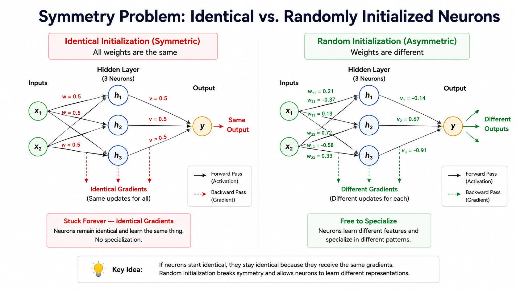
যদি কোনো হিডেন লেয়ারে ঢোকা প্রতিটি ওয়েটের মান একই হয়, তবে ওই লেয়ারের প্রতিটি নিউরন যেকোনো ইনপুট থেকে একটি হুবহু একই প্রি-অ্যাক্টিভেশন ক্যালকুলেট করবে। হুবহু একই প্রি-অ্যাক্টিভেশনগুলো হুবহু একই অ্যাক্টিভেশন তৈরি করে। হুবহু একই অ্যাক্টিভেশনগুলো লসের ক্ষেত্রে হুবহু একই অবদান রাখে, যার মানে হলো ব্যাকপ্রোপাগেশনের সময় ওই লেয়ারের প্রতিটি নিউরন একটি হুবহু একই গ্রেডিয়েন্ট পায়। যেহেতু আপডেট রুলটি এই হুবহু একই গ্রেডিয়েন্টটিকে আগে থেকেই একরকম হয়ে থাকা ওয়েটগুলোর ওপর প্রয়োগ করে, তাই আপডেটের পরেও ওয়েটগুলো ঠিক একই থেকে যায় — এবং প্রতিটি ইপকে (epoch) ঠিক এটাই বারবার ঘটতে থাকে, অনন্তকাল ধরে। সংখ্যক নিউরনের একটি লেয়ার তখন বার ডুপ্লিকেট করা একটিমাত্র নিউরনের মতো আচরণ করতে থাকে, যা চিরস্থায়ীভাবে নেটওয়ার্কের শেখার ক্ষমতার বা representational capacity-এর প্রায় সবটুকু নষ্ট করে দেয়।
এর সমাধান হলো ওয়েটগুলোকে র্যান্ডমভাবে বা randomly ইনিশিয়ালাইজ করা, যাতে প্রতিটি নিউরন ইনপুটের কিছুটা আলাদা একটি ফাংশন ক্যালকুলেট করার মাধ্যমে শুরু করতে পারে, একটি কিছুটা আলাদা গ্রেডিয়েন্ট পায় এবং তাই ট্রেনিং এগিয়ে যাওয়ার সাথে সাথে নিজেকে আলাদা কাজে দক্ষ বা specialize করার স্বাধীনতা পায়। মজার ব্যাপার হলো, বায়াসগুলোর (biases) ক্ষেত্রে এমনটা করার দরকার হয় না — এদেরকে সাধারণত ঠিক শূন্য (zero) দিয়েই ইনিশিয়ালাইজ করা হয়, কারণ নিউরনগুলোর ভেতরের সিমেট্রি ভাঙার জন্য শুধু র্যান্ডম ওয়েটগুলোই যথেষ্ট।
র্যান্ডমনেসের স্কেল কেন এত গুরুত্বপূর্ণ (Why the Scale of Randomness Matters)
শুধু কিছু র্যান্ডম নম্বর টেনে আনলেই গল্পের শেষ হয় না — ওই র্যান্ডমনেসের ভ্যারিয়েন্স (variance)-টি খুব ভেবেচিন্তে বেছে নিতে হয়।
খুব বড় বা খুব ছোট — দুটিই ট্রেনিংকে ভেঙে দেয়
যদি শুরুর দিকের ওয়েটগুলো খুব বড় হয়, তবে প্রি-অ্যাক্টিভেশনগুলো এক লেয়ার থেকে আরেক লেয়ারে যাওয়ার সময় আরও বড় হতে থাকে। সিগময়েড এবং ট্যানএইচ (tanh)-এর মতো স্যাচুরেটিং অ্যাক্টিভেশনগুলোর জন্য, এটি একদম প্রথম ফরওয়ার্ড পাস থেকেই নিউরনগুলোকে তাদের ফ্ল্যাট বা সমতল অঞ্চলে ঠেলে দেয়, যা ট্রেনিং শুরু হওয়ার সুযোগ পাওয়ার আগেই ভ্যানিশিং গ্রেডিয়েন্ট (vanishing gradients) তৈরি করে। আর যদি শুরুর দিকের ওয়েটগুলো খুব ছোট হয়, তবে অ্যাক্টিভেশনগুলো লেয়ারে লেয়ারে শূন্যের দিকে ছোট হতে থাকে — যা আবারও নেটওয়ার্ককে গ্রেডিয়েন্ট সিগন্যাল থেকে বঞ্চিত করে, অথবা প্রতিটি নিউরনকে একটি প্রায়-লিনিয়ার বা রৈখিক এবং অপ্রয়োজনীয় অঞ্চলে আটকে রাখে।
এর একটি যৌক্তিক সমাধান হলো এমন একটি র্যান্ডম ডিস্ট্রিবিউশন বেছে নেওয়া, যার ভ্যারিয়েন্সটি গাণিতিকভাবে বের করা হয়, যাতে ডেটা প্রতিটি লেয়ারের ভেতর দিয়ে যাওয়ার সময় অ্যাক্টিভেশনের ভ্যারিয়েন্স — এবং একইভাবে, পেছনের দিকে বয়ে চলা গ্রেডিয়েন্টের ভ্যারিয়েন্স — মোটামুটি স্থির থাকে, লেয়ার থেকে লেয়ারে যাওয়ার সময় এটি যেন খুব বড় বা খুব ছোট হয়ে না যায়। ঠিক এই গাণিতিক হিসাব বা derivation-টাই নিচের স্কিমগুলো (schemes) করে থাকে, যার প্রতিটি আলাদা আলাদা অ্যাক্টিভেশন ফাংশনের জন্য বিশেষভাবে তৈরি করা।
জাভিয়ার (গ্লোরোট) ইনিশিয়ালাইজেশন (Xavier / Glorot Initialization)
যেখানে: এবং হলো ওই লেয়ারের ইনপুট এবং আউটপুট ইউনিটের সংখ্যা।
পেছনের যুক্তি বা Intuition: সিগন্যাল প্রতিটি লেয়ারের ভেতর দিয়ে প্রবাহিত হওয়ার সময় অ্যাক্টিভেশনের ভ্যারিয়েন্স — এবং একইভাবে, ব্যাকওয়ার্ড পাসের সময় গ্রেডিয়েন্টের ভ্যারিয়েন্স — যেন মোটামুটি স্থির বা কনস্ট্যান্ট থাকে, সেই শর্ত ধরে নিয়ে জাভিয়ার ইনিশিয়ালাইজেশনকে ম্যাথমেটিক্যালি বা গাণিতিকভাবে ডেরাইভ বা প্রতিপাদন করা হয়। কোনো লেয়ারের প্রি-অ্যাক্টিভেশনের ভ্যারিয়েন্সকে তার আগের লেয়ারের অ্যাক্টিভেশনের ভ্যারিয়েন্সের সমান ধরে নিলে এবং স্বাধীন র্যান্ডম ভ্যারিয়েবলগুলোর যোগফলের ভ্যারিয়েন্সের অ্যালজেবরা বা বীজগণিতের হিসেব কষলে, তা সরাসরি এই ফর্মুলাটিতে এসে দাঁড়ায়। এটি সিগময়েড এবং ট্যানএইচ-এর মতো এমন সব অ্যাক্টিভেশনের জন্য ডিজাইন করা হয়েছে, যাদের ডেরিভেটিভ (derivative) খুব ভালোভাবে আচরণ করে এবং শূন্যের কাছাকাছি মোটামুটি সিমেট্রিক বা প্রতিসম থাকে।
হে (কাইমিং) ইনিশিয়ালাইজেশন (He / Kaiming Initialization)
এটি কেন জাভিয়ার থেকে আলাদা: রেলু (ReLU) তার ইনপুটের মোটামুটি অর্ধেক অংশকে শূন্য করে দেয় — প্রতিটি নেগেটিভ প্রি-অ্যাক্টিভেশনকে কেটে ঠিক শূন্য বানিয়ে দেয় — যা একটি লিনিয়ার বা সিমেট্রিক অ্যাক্টিভেশনের তুলনায় সামনের দিকে এগিয়ে যাওয়া অ্যাক্টিভেশনের ভ্যারিয়েন্সকে কার্যকরভাবে অর্ধেক করে দেয়। হে (He) ইনিশিয়ালাইজেশন ভ্যারিয়েন্সকে দ্বিগুণ করে (, যেখানে একই আকারের লেয়ারের জন্য জাভিয়ারের ভ্যারিয়েন্স ছিল ) এই ঘাটতিটুকু পুষিয়ে দেয়, যা বিশেষভাবে ReLU-পরিবারের অ্যাক্টিভেশনগুলোর কার্যকর সিগন্যাল ভ্যারিয়েন্সকে স্থির রাখে।
ইন্টারভিউয়ের একটি প্রিয় প্রশ্ন (A favorite interview question)
"হে (He) ইনিশিয়ালাইজেশনে কেন জাভিয়ার (Xavier)-এর থেকে আলাদা ফর্মুলা ব্যবহার করা হয়?" এর খুব পরিষ্কার উত্তরটি হলো: ReLU তার ইনপুটের প্রায় অর্ধেককে শূন্য করে দেয়, যা একটি সিমেট্রিক অ্যাক্টিভেশনের তুলনায় ফরওয়ার্ড-পাসের ভ্যারিয়েন্সকে অর্ধেক করে ফেলে; ইনিশিয়ালাইজেশনের ভ্যারিয়েন্সকে দ্বিগুণ করলে তা এই ক্ষতির ঠিকঠাক ক্ষতিপূরণ দেয় এবং লেয়ার থেকে লেয়ারে সিগন্যালের মাত্রা বা ম্যাগনিটিউড (magnitude) স্থির রাখে। জাভিয়ার ধরে নেয় যে অ্যাক্টিভেশনটি tanh বা সিগময়েডের মতো একটি সিমেট্রিক এবং নন-জিরোয়িং (non-zeroing) অ্যাক্টিভেশন, যেখানে এমন কোনো ক্ষতিপূরণের দরকার হয় না।
লেকুন ইনিশিয়ালাইজেশন (LeCun Initialization)
যাদের জন্য ডিজাইন করা: এটি SELU অ্যাক্টিভেশনের জন্য ডিজাইন করা হয়েছে, যার সেল্ফ-নর্মালাইজিং (self-normalizing) প্রপার্টি — অর্থাৎ অ্যাক্টিভেশনগুলো লেয়ারের ভেতর দিয়ে যাওয়ার সময় নিজে থেকেই জিরো মিন (zero mean) এবং ইউনিট ভ্যারিয়েন্সের (unit variance) দিকে এগোতে থাকে — গাণিতিকভাবে এমন একটি নির্দিষ্ট ধারণার ওপর ভিত্তি করে প্রতিপাদন করা হয়েছে যেখানে ওয়েটগুলোকে ঠিক এভাবেই ইনিশিয়ালাইজ করা হয়। SELU-এর সাথে লেকুন ইনিশিয়ালাইজেশন ব্যবহার না করলে ওই সেল্ফ-নর্মালাইজিং গ্যারান্টিটি আর কাজ করে না।
হাতে-কলমে সংখ্যাগত তুলনা: জাভিয়ার বনাম হে (Worked Numeric Comparison: Xavier vs. He)
একটি আকারের লেয়ার নিয়ে ভাবি, অর্থাৎ ।
- জাভিয়ার: ভ্যারিয়েন্স , অর্থাৎ স্ট্যান্ডার্ড ডেভিয়েশন ।
- হে: ভ্যারিয়েন্স , অর্থাৎ স্ট্যান্ডার্ড ডেভিয়েশন ।
দুটি সংখ্যাই ছোট দেখতে হলেও, হে-এর স্ট্যান্ডার্ড ডেভিয়েশন জাভিয়ারের চেয়ে প্রায় গুণ বড়। এখন কল্পনা করুন একটি ReLU নেটওয়ার্কে ভুল করে জাভিয়ার ইনিশিয়ালাইজেশন ব্যবহার করা হলো: প্রতিটি লেয়ারে ReLU ইনপুটের প্রায় অর্ধেক শূন্য করে দেয়, আর ইনিশিয়ালাইজেশনও এমনিতে একটু কম ভ্যারিয়েন্স দিচ্ছে। ফলাফল হলো প্রতিটি লেয়ারে সিগন্যালের ভ্যারিয়েন্স ধারাবাহিকভাবে সংকুচিত হতে থাকে — ১০টি লেয়ার পার হওয়ার পর অ্যাক্টিভেশনের ভ্যারিয়েন্স মূল মানের তুলনায় প্রায় গুণ ছোট হয়ে যেতে পারে, যা কার্যত ভ্যানিশিং গ্রেডিয়েন্টের একটি ধীরগতির সংস্করণ।
একটি দ্রুত স্যানিটি-চেক
নতুন কোনো আর্কিটেকচার লেখার পর ট্রেনিং শুরু করার আগে, প্রতিটি লেয়ারের আউটপুটের স্ট্যান্ডার্ড ডেভিয়েশন প্রিন্ট করে দেখুন (একটি র্যান্ডম ব্যাচ ফরওয়ার্ড পাস করিয়ে)। যদি এই সংখ্যাগুলো লেয়ার থেকে লেয়ারে ধারাবাহিকভাবে ছোট হতে থাকে বা বড় হতে থাকে, তবে সেটিই একটি পরিষ্কার সংকেত যে ইনিশিয়ালাইজেশন স্কিমটি ব্যবহৃত অ্যাক্টিভেশন ফাংশনের সাথে মানানসই নয়।
ইনিশিয়ালাইজেশনের সাথে ব্যাচ নরমালাইজেশনের সম্পর্ক (Interaction With Batch Normalization)
যেসব লেয়ারের ঠিক পরেই ব্যাচ নরমালাইজেশন (Batch Normalization) বসানো থাকে, সেখানে ইনিশিয়ালাইজেশনের সূক্ষ্ম ভ্যারিয়েন্স হিসাব অনেকটাই কম সংবেদনশীল হয়ে পড়ে — কারণ BatchNorm নিজেই প্রতিটি মিনি-ব্যাচে অ্যাক্টিভেশনের ভ্যারিয়েন্সকে জোর করে প্রায় স্থির (unit variance) রেখে দেয়, লেয়ারের ইনপুট ওয়েটের স্কেল যাই হোক না কেন। এর মানে এই নয় যে ইনিশিয়ালাইজেশন আর গুরুত্বপূর্ণ নয়; বরং এর মানে হলো BatchNorm একটি সুরক্ষাবলয় বা সেফটি নেট হিসেবে কাজ করে, যা একটি মাঝারি মানের ভুল ইনিশিয়ালাইজেশনের প্রভাবকে অনেকটাই নিরপেক্ষ করে দিতে পারে — যদিও তা সিমেট্রি ভাঙার মৌলিক প্রয়োজনীয়তাকে (র্যান্ডম ওয়েট) মোটেও প্রতিস্থাপন করে না।
এক নজরে তুলনা (Comparison at a Glance)
| স্কিম (Scheme) | ভ্যারিয়েন্স (Variance) | যাদের জন্য রেকমেন্ড করা হয় (Recommended For) |
|---|---|---|
| জিরো বা ধ্রুবক (Zero / constant) | 0 | ওয়েটের জন্য কখনোই না (সিমেট্রির সমস্যা); বায়াসের জন্য ঠিক আছে |
| নেইভ র্যান্ডম, যেমন ছোট ইউনিফর্ম (Naive random) | ইচ্ছেমতো, স্কেল করা নয় (Arbitrary, unscaled) | রেকমেন্ড করা হয় না — এর স্কেলটি যুক্তিসঙ্গত নয় |
| জাভিয়ার / গ্লোরোট (Xavier / Glorot) | সিগময়েড (Sigmoid), ট্যানএইচ (tanh) | |
| হে / কাইমিং (He / Kaiming) | রেলু (ReLU), লিকি রেলু (Leaky ReLU), ইএলইউ (ELU) | |
| লেকুন (LeCun) | সেলু (SELU) |
Implementation
python
xavier_init এবং he_init ফাংশন দুটির মধ্যে পার্থক্য শুধু ভ্যারিয়েন্স ফর্মুলার ডিনোমিনেটর (denominator) বা হর হিসেবে কোনটা ব্যবহার করা হচ্ছে তাতেই — র্যান্ডম ম্যাট্রিক্স তৈরি করার বাকি সবকিছুই হুবহু এক। খেয়াল করুন যে দুটি ফাংশনই n_in এবং n_out-কে হার্ডকোড (hardcode) করার বদলে সরাসরি আর্গুমেন্ট বা ইনপুট হিসেবে নেয়, কারণ সঠিক ভ্যারিয়েন্স হলো লেয়ারের আকার বা shape-এর একটি ফাংশন, এটি কোনো ইউনিভার্সাল বা চিরন্তন কনস্ট্যান্ট নয়। নিচের কমেন্ট করে রাখা লাইনগুলো বাস্তব প্রজেক্টের জন্য মনে রাখা খুব জরুরি: প্রোডাকশনের কোডে প্রায় কখনোই এই ফর্মুলাগুলো নিজে হাতে লেখা হয় না, কারণ প্রতিটি বড় ফ্রেমওয়ার্কই এগুলোকে এক লাইনের kernel_initializer অথবা nn.init কল হিসেবে দিয়ে রাখে।
কাজের ক্ষেত্রে সাধারণ একটি নিয়ম (Practical rule of thumb)
যে লেয়ারের পর ReLU-পরিবারের কোনো অ্যাক্টিভেশন থাকবে, সেখানে হে (He) ইনিশিয়ালাইজেশন ব্যবহার করুন — আধুনিক MLP-গুলোতে এটিই সবচেয়ে কমন — আর যে লেয়ারের পর সিগময়েড বা ট্যানএইচ থাকবে, সেখানে জাভিয়ার (Xavier) ইনিশিয়ালাইজেশন ব্যবহার করুন। প্রোডাকশনের কাজে নিজে হাতে এদের কোনোটি ইমপ্লিমেন্ট করার খুব একটা দরকার পড়ে না, কিন্তু এর পেছনের গাণিতিক কারণ বা derivation-টি বুঝতে পারলেই আপনি একটি বাজে ইনিশিয়ালাইজেশন থেকে তৈরি হওয়া ট্রেনিংয়ের অস্থিতিশীলতা বা instability খুব সহজেই ধরে ফেলতে পারবেন।
মূল বিষয়গুলো (Key Takeaways)
Key Takeaways
- ওয়েট-কে শূন্য (বা অন্য কোনো একই কনস্ট্যান্ট) দিয়ে ইনিশিয়ালাইজ করলে সিমেট্রির সমস্যা বা symmetry problem দেখা দেয়: লেয়ারের প্রতিটি নিউরন ওই লেয়ারের অন্য সব নিউরনের মতো হুবহু একই থেকে যায়, ট্রেনিং যত লম্বাই হোক না কেন, তা অনন্তকাল ধরে চলতে থাকে।
- একটিমাত্র পারসেপ্ট্রনের কখনো এই সমস্যাটি হয়নি কারণ তার লেয়ারে একে অপরের থেকে আলাদা করে চেনার জন্য অন্য কোনো "ভাই-বোন" বা sibling নিউরন নেই — সমস্যাটি কেবল তখনই দেখা দেয় যখন কোনো লেয়ারে একের বেশি নিউরন থাকে।
- ওয়েটগুলোকে অবশ্যই র্যান্ডমভাবে ইনিশিয়ালাইজ করতে হবে, এবং একদম প্রথম ফরওয়ার্ড পাস থেকেই অ্যাক্টিভেশনগুলো যাতে ভ্যানিশিং (vanishing) বা এক্সপ্লোডিং (exploding) না হয়ে যায়, সেজন্য ওই র্যান্ডমনেসের ভ্যারিয়েন্সটি র্যান্ডমনেসের মতোই সমান গুরুত্বপূর্ণ।
- জাভিয়ার/গ্লোরোট ইনিশিয়ালাইজেশন () সিগময়েড এবং ট্যানএইচ-এর মতো সিমেট্রিক এবং নন-জিরোয়িং (non-zeroing) অ্যাক্টিভেশনগুলোর জন্য ডিজাইন করা।
- হে/কাইমিং ইনিশিয়ালাইজেশন () ReLU-এর ইনপুটের অর্ধেক শূন্য হয়ে যাওয়ার ঘাটতিকে পূরণ করে এবং এটি ReLU-পরিবারের অ্যাক্টিভেশনগুলোর জন্য স্ট্যান্ডার্ড ডিফল্ট।
- SELU-এর সেল্ফ-নর্মালাইজিং (self-normalizing) প্রপার্টি গাণিতিকভাবে কাজ করার জন্য লেকুন ইনিশিয়ালাইজেশন () অবশ্যই দরকার।
- বায়াসগুলোকে সাধারণত কোনো ঝামেলা ছাড়াই শূন্য দিয়ে ইনিশিয়ালাইজ করা হয়, কারণ শুধু র্যান্ডম ওয়েটগুলোই সিমেট্রি ভাঙার জন্য যথেষ্ট।
সাধারণ ভুল ধারণা (Common Mistakes)
ধরে নেওয়া যে জিরো-ইনিশিয়ালাইজেশন সবসময় নিরাপদ (Assuming zero-initialization is always safe)
পারসেপ্ট্রনের মতো একটিমাত্র নিউরনের মডেলের জন্য জিরো-ইনিশিয়ালাইজেশন ঠিক আছে, কিন্তু একের বেশি নিউরন থাকা যেকোনো হিডেন লেয়ারের জন্য এটি এক কথায় সর্বনাশা। লেয়ারের পর লেয়ার সাজানো শুরু করার সময় ভুল করে এই অভ্যাসটি টেনে আনা খুব সহজ।
অ্যাক্টিভেশন ফাংশনের জন্য ভুল ইনিশিয়ালাইজেশন ব্যবহার করা (Using the wrong initialization for the activation function)
ReLU লেয়ারের আগে জাভিয়ার ইনিশিয়ালাইজেশন প্রয়োগ করলে (অথবা tanh লেয়ারের আগে হে ইনিশিয়ালাইজেশন প্রয়োগ করলে) তা হয়তো সরাসরি কোনো ক্র্যাশ (crash) করাবে না, কিন্তু এটি নীরবে একটি মিসম্যাচড বা ভুল সিগন্যাল ভ্যারিয়েন্স তৈরি করে, যা পরে অপ্রত্যাশিতভাবে ধীরগতির বা অস্থিতিশীল ট্রেনিং হিসেবে দেখা দেয় এবং এর আসল কারণ খুঁজে বের করা খুব কঠিন হয়ে পড়ে।
ভ্যানিশিং/এক্সপ্লোডিং গ্রেডিয়েন্ট ডিবাগ করার সময় ইনিশিয়ালাইজেশনকে এড়িয়ে যাওয়া (Ignoring initialization when debugging vanishing/exploding gradients)
যখন ট্রেনিংয়ের একদম প্রথম ধাপেই — কোনো অপ্টিমাইজারের সমস্যা বা আর্কিটেকচারের ত্রুটির কারণে এমনটা হতে পারে তা বোঝার আগেই — গ্রেডিয়েন্ট ভ্যানিশ (vanish) বা এক্সপ্লোড (explode) করে, তখন সবার আগে যে জায়গাগুলোতে নজর দিতে হয়, তার মধ্যে ইনিশিয়ালাইজেশন স্কিমটি অন্যতম, এটি শেষের দিকের কোনো বিষয় নয়।
ইনিশিয়ালাইজেশনের ভ্যারিয়েন্স মনে রেখে ফাইন-টিউনিংয়ের (fine-tuning) সময় নতুন লেয়ার যোগ করা (Adding new layers during fine-tuning without matching variance)
কোনো প্রি-ট্রেইনড (pre-trained) নেটওয়ার্কের ওপর নতুন একটি হেড বা লেয়ার যোগ করার সময়, সেই নতুন লেয়ারটিকে বাকি নেটওয়ার্কের সাথে মানানসই একটি স্কিম দিয়ে ইনিশিয়ালাইজ করতে ভুলে গেলে (যেমন ডিফল্ট ইনিশিয়ালাইজেশনে রেখে দিলে), নতুন লেয়ারের গ্রেডিয়েন্ট বাকি নেটওয়ার্কের তুলনায় অস্বাভাবিক বড় বা ছোট হয়ে যেতে পারে, যা ফাইন-টিউনিংয়ের প্রথম কয়েক ধাপকে অস্থিতিশীল করে তোলে।
ইনিশিয়ালাইজেশনকে ট্রেনিংয়ের একটি ওয়ান-টাইম বা একবারের বিষয় মনে করা (Treating initialization as a one-time, forgettable step)
একবার ট্রেনিং শুরু হয়ে গেলে ইনিশিয়ালাইজেশন যেন আর কোনো ভূমিকাই রাখে না — এমনটা মনে করা একটি সাধারণ ভুল ধারণা। ইনিশিয়ালাইজেশন শুধু ট্রেনিংয়ের শুরুর বিন্দুটি ঠিক করে দেয় না, বরং এটি লস ল্যান্ডস্কেপের ঠিক কোন অংশ থেকে অপ্টিমাইজেশন শুরু হচ্ছে তা নির্ধারণ করে, যা শেষ পর্যন্ত মডেলটি কোন লোকাল মিনিমাতে গিয়ে থামবে তার ওপরও প্রভাব ফেলতে পারে — বিশেষ করে নন-কনভেক্স (non-convex) লস সারফেসে, যেখানে একাধিক ভিন্ন মানের মিনিমা থাকতে পারে।
ইন্টারভিউ কর্নার (Interview Corner)
Quick Check
বাস্তবে এটি কোথায় দেখা যায় (Where This Shows Up in Practice)
প্রতিটি বড় ডিপ লার্নিং ফ্রেমওয়ার্ক নিজে থেকেই নতুন লেয়ারগুলোর জন্য একটি যৌক্তিক বা সেন্সিবল ইনিশিয়ালাইজেশন স্কিম ঠিক করে দেয় — Keras-এর Dense লেয়ার ডিফল্ট হিসেবে Glorot uniform ব্যবহার করে, PyTorch-এর nn.Linear ডিফল্ট হিসেবে Kaiming-ভিত্তিক একটি স্কিম ব্যবহার করে — কারণ ঠিক এই ধাপটিতে ভুল করাটাই হলো ট্রেনিং ব্যর্থ হওয়ার সবচেয়ে সাধারণ এবং খুব সহজেই এড়ানো যায় এমন একটি কারণ। এই ডিফল্টগুলো কেন আছে তা বুঝতে পারলেই আপনি ধরে ফেলতে পারবেন যে কখন এই ডিফল্টটি আপনার আর্কিটেকচারের জন্য ভুল (উদাহরণস্বরূপ, যখনই আপনি কোনো সিগময়েড হিডেন লেয়ার বদলে ReLU ব্যবহার করবেন, তখনই হে (He) ইনিশিয়ালাইজেশনে চলে যাওয়া), আর ঠিক এ ধরনের মৌলিক ডিটেইল বা খুঁটিনাটিগুলোই একটি মসৃণভাবে ট্রেন হওয়া মডেলকে এমন একটি মডেল থেকে আলাদা করে যা রহস্যজনকভাবে কখনোই কনভার্জ করে না।